We work with numerical data in our Excel worksheet all the time. We perform various operations on them. Finding Summation is the most common task of them all. But, decimals on those data can bring a deviation from the correct sum result. In this article, we’ll show you the effective ways to Round Excel Data to Make Summations Correct.
How to Round Excel Data to Make Summations Correct: 7 Easy Methods
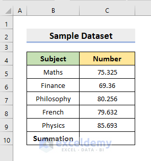
To illustrate, we’ll use a sample dataset as an example. For instance, the following dataset represents the Subjects and the obtained Numbers of a student. The numbers are in decimal format. Here, we’ll round the numbers to integer, single decimal, and two decimal formats.
1. Excel ‘Decrease Decimal’ Feature to Round Data for Making Precise Summations
We can manually decrease decimal places in a number value. In our first method, we’ll perform the task to round the data to a whole number. Therefore, follow the steps below.
STEPS:
- First, select the range C5:C9.
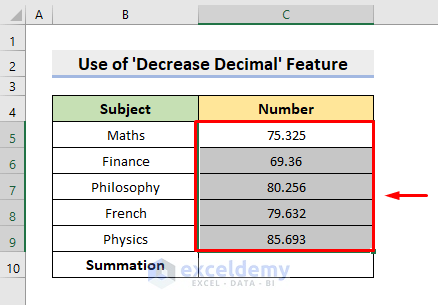
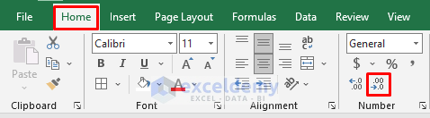
- Then, under the Home tab, click the Decrease Decimal feature (marked in the following image) 3 times (to convert it to integers).
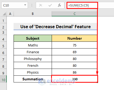
- As a result, it’ll return the whole numbers as it’s shown below.

- Finally, select cell C10 and use the AutoSum feature to find the total.
- Thus, you’ll get the correct result.
Read More: How to Round a Formula with SUM in Excel
2. Correct Sum Total after Rounding Excel Data with Number Format
We can use the Number Format in Excel to round the numbers to a 2 decimal place. So, learn the following steps to carry out the operation.
STEPS:
- Firstly, select C5:C9.
- After that, press the Number format in the Number section.

- Subsequently, in cell C10, press the AutoSum.
- Lastly, it’ll return the total in 2 Decimal format (27).

Read More: How to Roundup a Formula Result in Excel
3. Use Format Cells to Round for Finding Exact Total
Moreover, we can apply the Format Cells feature in Excel to round numbers to our requirement. Hence, follow the below process for using Format Cells to Round for Finding Exact Total.
STEPS:
- First of all, press the keys Ctrl and 1 simultaneously after selecting the range C5:C9.
- Consequently, the Format Cells dialog box will pop out.
- Select 0 (for integer) in Decimal places from the Number tab.
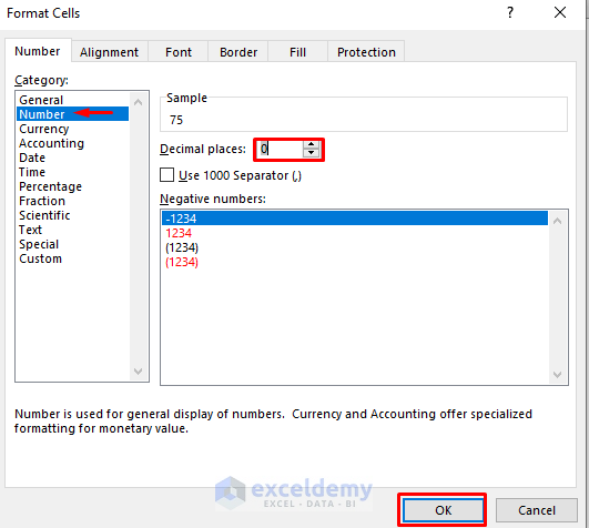
- Now, press OK.
- As a result, it’ll return the numbers in the desired format.
- Next, use AutoSum in cell C10 and you’ll see the correct summation.

4. Apply ROUND Function to Make Summations Correct
However, Excel provides the ROUND Function for rounding the data. In this method, we’ll make use of the function. Therefore, learn the following process to perform the task.
STEPS:
- Select cell D5 at first.
- Here, type the formula:
=ROUND(C5,0)- Then, press Enter.
- Afterward, use AutoFill to complete the series.
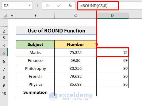
NOTE: In the ROUND function argument, we specified 0 to convert it to an integer. You can input any other number (1,2 etc.) to convert them to other decimal values.
- Subsequently, in cell C10, type the formula:
=SUM(D5:D9)- At last, press Enter to return the precise sum result.

5. Excel ROUNDUP Function for Rounding Data
We have another function named the ROUNDUP Function to carry out a similar operation. This function rounds up a number to a decimal format away from the Zero. So, see the steps carefully for applying ROUNDUP Function to Round Data.
STEPS:
- In the beginning, select cell D5 to type the formula:
=ROUNDUP(C5,1)- Press Enter and use AutoFill to return the values to a single decimal format.
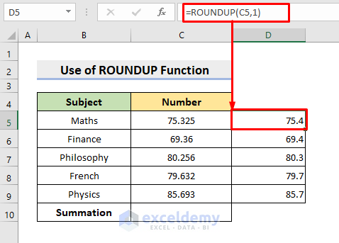
NOTE: In the ROUNDUP function argument, we specified 1 to convert it to a single decimal. Input any other number (0,2 etc.) to convert them to other decimal values.
- After that, select cell C10 to type the formula:
=SUM(D5:D9)- In the end, press Enter. Thus, you’ll see the exact total.

Read More: How to Round up Decimals in Excel
6. Find Exact Sum Using ROUNDDOWN Function
Additionally, to round a number down towards Zero, we can apply the ROUNDDOWN Function. Now, go through the below process to Round Excel Data to Make Summations Correct.
STEPS:
- Firstly, type the below formula in cell D5:
=ROUNDDOWN(C5,1)- Then, press Enter.
- Consequently, fill the series with AutoFill.
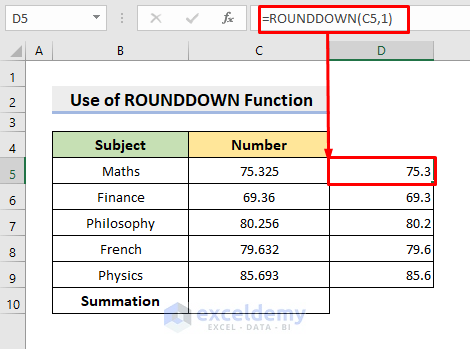
NOTE: In the ROUNDDOWN function argument, we specified 1 to round it down to a single decimal. Input any other number (0,2 etc.) to convert them to other decimal values.
- Now, type the formula in the cell C10:
=SUM(D5:D9)- Lastly, press Enter to get the correct summation result.

Read More: How to Set Decimal Places in Excel with Formula
7. Round Data with Excel TRUNC Function to Find Precise Sum
In our last method, we’ll use the Excel TRUNC Function. This function truncates a number to an integer removing the decimal parts. Hence, follow the steps to Find the Precise Sum.
STEPS:
- Select cell D5 at first.
- Next, type the formula:
=TRUNC(C5)- Press Enter and use AutoFill.
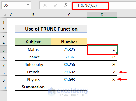
NOTE: This function simply ignores the decimal parts and returns the whole numbers. For this reason, D8 and D9 cells are different from our previous examples.
- Eventually, in cell C10, type the formula:
=SUM(D5:D9)- Press Enter. As a result, you’ll get an accurate sum.

Read More: Round off Formula in Excel Invoice
Download Practice Workbook
Download the following workbook to practice by yourself.
Conclusion
Henceforth, you will be able to Round Excel Data to Make Summations Correct by following the above-described methods. Keep using them and let us know if you have more ways to do the task. Follow the ExcelDemy website for more articles like this. Don’t forget to drop comments, suggestions, or queries if you have any in the comment section below.
Related Articles
- How to Add ROUND Formula to Multiple Cells in Excel
- How to Round Numbers in Excel Without Formula
- How to Round Percentages in Excel
- How to Set Rounding Precision in Excel
- How to Round a Multiplication Formula in Excel
<< Go Back to Rounding in Excel | Number Format | Learn Excel
Get FREE Advanced Excel Exercises with Solutions!
