In Excel, you may come across repetitive tasks often. To number rows is one of these tasks which can be a time-consuming one. There are several ways of performing this task in a time-saving manner.
Our agenda for today is to show you how to number rows in Excel. Before diving into the session, let’s get to know about the dataset that is the base of our examples.
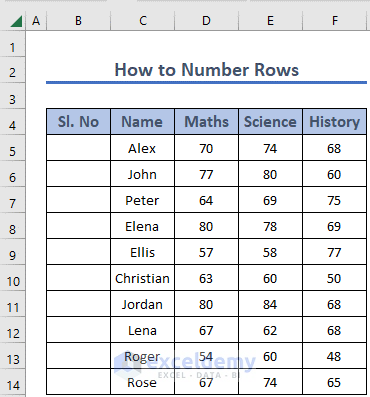
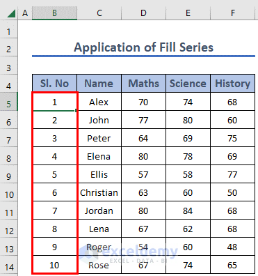
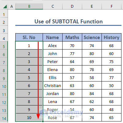
Here we have listed a few students and their scores in three courses. Using this dataset, we will show you how to number rows.

Note that this is a basic table to keep things simple. You may encounter a much larger and more complex dataset in a practical scenario.
How to Number Rows in Excel: 9 Suitable Ways
As we have mentioned there are several methods for numbering rows. Let’s explore them.
For example, we will add the serial number to each of the rows here.
1. Use the AutoFill Feature to Number Rows in Excel
We can use the Excel AutoFill feature to number rows.
Steps:
- First of all, you need to insert a couple of numbers in the first two cells.
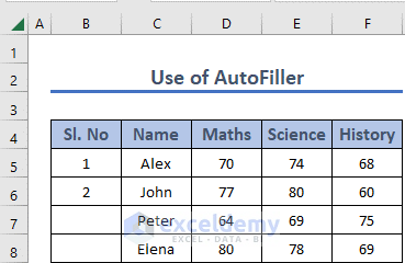
- We need to insert two rows so that Excel can understand the pattern.
- Then select both rows together.
- After selecting the rows you will see a tiny rectangle box at the bottom right corner of selected cells. This is called Fill Handle.
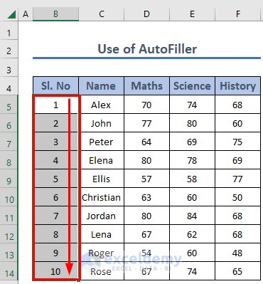
- Double-click there or drag it down to the remaining rows.
- You will find numbers for the rows.
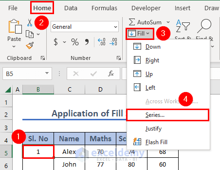
2. Apply Fill Series Feature to Number Rows in Excel
Another worth mentioning feature is the Fill Series. We can use this feature for numbering the rows.
Steps:
- Insert 1 at the first cell.
- Now go to the Home tab.
- Then, select Fill.
- From the drop-down, select Series.
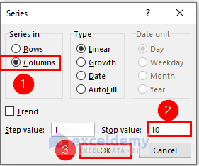
- You will find a Series dialog box in front of you. From there, select Columns in Series in This denotes that the series will be filled within a single column.
- Set the Step Value and Stop Value as your situation demands (here we have set 1 and 10 for these respectively).
- Then click OK.
- You will find numbers for the rows.
3. Add 1 to Previous Cell
Now, I will add 1 to the previous cells to number rows.
Steps:
- Write 1 in B5.
- Then, write down the following formula in B6.
=B5+1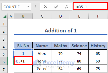
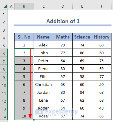
- Then, press ENTER to get the output.

- Finally, use Fill Handle to AutoFill up to B14.
4. Use ROW Function to Number Rows in Excel
We can use several Excel basic functions for numbering the rows. The ROW function can be one of those functions.
Steps:
- Go to B5 and write down the following formula.
=ROW(B1)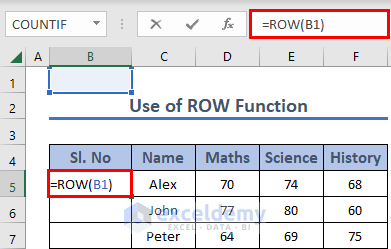
- Since we want to number it from 1, we inserted the first row (which can be from any column) within it.
- Then, press ENTER to get the output.
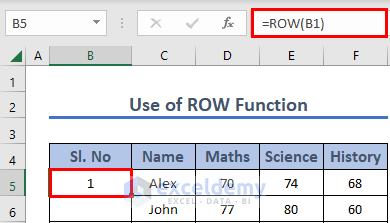
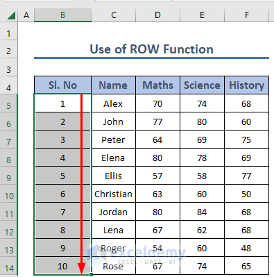
- Finally, use Fill Handle to AutoFill up to B14.
Read More: How to Create Rows within a Cell in Excel
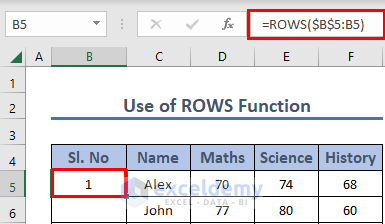
5. Apply ROWS Function
There is a ROW family function called ROWS. The ROWS function returns the count of rows in a given reference.
Steps:
- Go to B5 and write down the following formula
=ROWS($B$5:B5)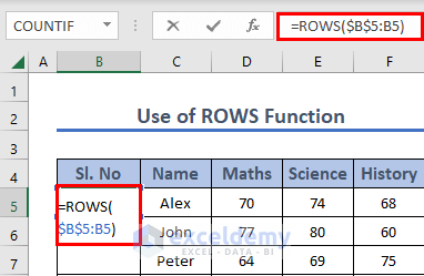
- This will provide the difference between the cells.
- We have provided the first cell number in absolute cell reference so that it remains the same for the next cells.
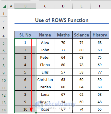
- Now, press ENTER to get the output.
- Then, use Fill Handle to AutoFill up to B14.
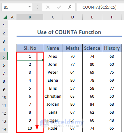
6. Use COUNTA Function to Number Rows
We can use the COUNTA function to number the rows in Excel. COUNTA counts the cells that are not empty. So this function will help number the rows that have values.
Steps:
- Go to B5 and write down the following formula
=COUNTA($C$5:C5)
- Then, press ENTER to get the output.

- After that, use Fill Handle to AutoFill up to B14.
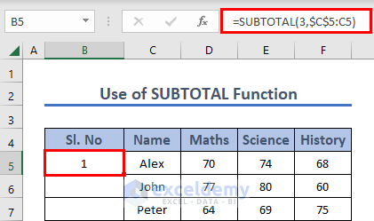
7. Apply SUBTOTAL Function
We can use the SUBTOTAL function for numbering rows. SUBTOTAL returns an aggregate result for supplied values. Several functional operations can be performed through this function.
Steps:
- Go to B5 and write down the following formula.
=SUBTOTAL(3,$C$5:C5)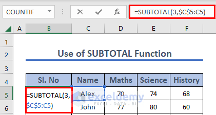
- 3 denotes the COUNTA operation. So, you can understand this formula performs like the previous section.
- Then, press ENTER to get the output.
- After that, use Fill Handle to AutoFill up to B14.
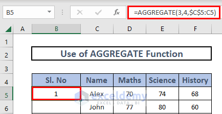
8. Use AGGREGATE Function to Number Rows
We can use the AGGREGATE function for numbering the rows. Like SUBTOTAL this AGGREGATE function also performs several functional operations.
Steps:
- Go to B5 and write down the following formula.
=AGGREGATE(3,4,$C$5:C5)
- 3 denotes the COUNTA operation and 4 is for ignoring nothing. So, you can understand this formula performs like the previous section.
- Then, press ENTER to get the output.
- After that, use Fill Handle to AutoFill up to B14.

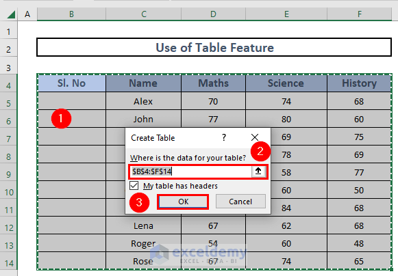
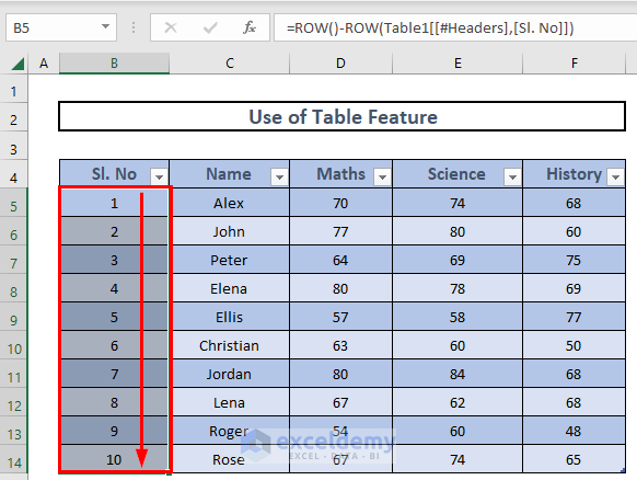
9. Create Table And Number Rows
Another approach to numbering rows is numbering through tables.
Steps:
- Select the entire list
- Then, press CTRL + T.
- Create Table box will appear.
- Check the box if your table has headers.
- Then, click OK.
- Then, go to B5 and write down the following formula
=ROW()-ROW(Table1[[#Headers],[Sl. No]])
Formula Breakdown
- Table1[[#Headers],[Sl. No]] → This is the reference with respect to the table headers.
- Output: “Sl. No”
- ROW(Table1[[#Headers],[Sl. No]]) → This will get you the Row number.
- Output: {4}
- ROW()-ROW(Table1[[#Headers],[Sl. No]]) → You will get the final result after subtracting the two row numbers.
- Output: {1}
- Then, press ENTER and AutoFill up to B14.
- Your output will look like this.
Download Practice Workbook
You are welcome to download the practice workbook from the following link.
Conclusion
That’s all for today. We have listed several methods to number rows in Excel. Hope you will find this helpful. Feel free to comment if anything seems difficult to comprehend. Let us know any other methods that we have missed here.
Related Articles
- How to Create Collapsible Rows in Excel
- How to Copy Every Nth Row in Excel
- How to Color Alternate Rows in Excel
- How to Expand and Collapse Rows in Excel
- How to Lock Rows in Excel
- How to Expand or Collapse Rows with Plus Sign in Excel
- How to Resize All Rows in Excel
<< Go Back to Rows in Excel | Learn Excel
Get FREE Advanced Excel Exercises with Solutions!
