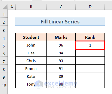
Method 1 – Fill a Linear Series in Excel in a Column
- Select cell D5.
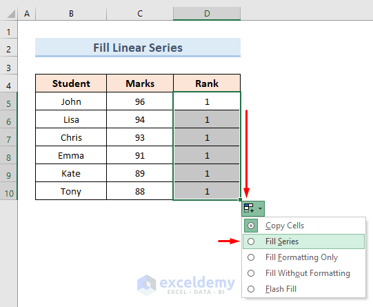
- Drag the Fill Handle tool to cell D10.
- From the dropdown of the right bottom corner select the option Fill Series.
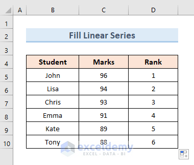
- See the series value in the Rank.
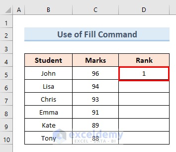
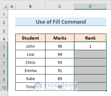
Method 2 – Use of Fill Command to Fill a Linear Series
- Select cell D5.
- Select the cell range (D5:D10).
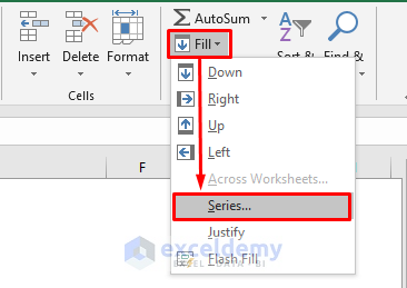
- Go to the Fill option under the editing section from the ribbon.
- Select the option Series.
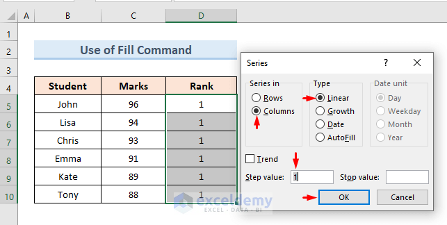
- A new dialogue box will open. Select the following options:
Series in: Columns
Type: Linear
Step Value: 1
- Press OK.
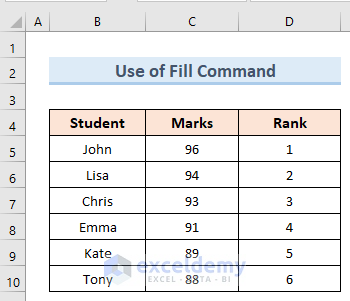
- Get the series of ranks in the Rank.
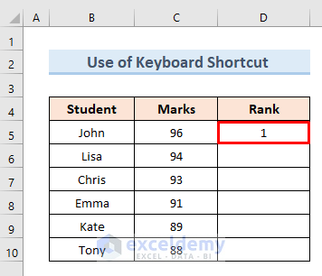
Method 3 – Fill Series with Keyboard Shortcut
- Select cell D5.
- Press Ctrl Drag the Fill Handle tool to cell D5.
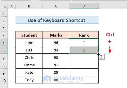
- Drag the Fill Handle from cell D6 to D10.
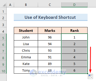
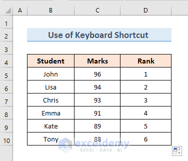
- See the series of ranks in Column D. You can autofill data in a column.
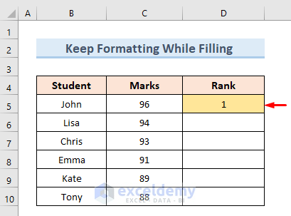
Method 4 – Keep Formatting While Filling a Series in Excel
- Select cell D5.
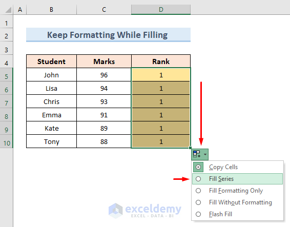
- Drag the Fill Handle tool to cell D10. From the dropdown of the AutoFill Options, select the option Fill Series.
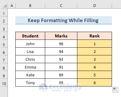
- Get the series value of ranks in the Rank.
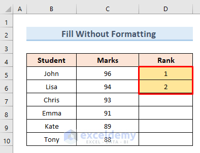
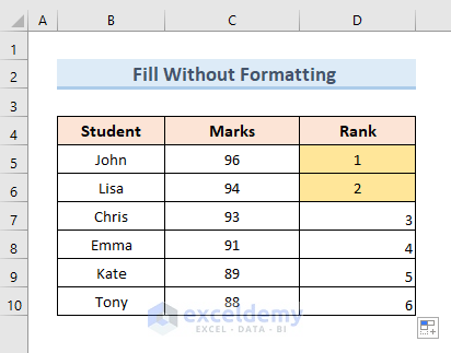
Method 5 – Filling a Series in Excel without Formatting
- Select cells D5 & D6.
-
- Drag the Fill Handle tool to cell D10.
- Select the option Fill Without Formatting from the dropdown of the AutoFill Options.
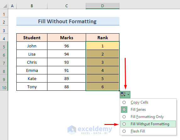
- See the value of the series without formatting.
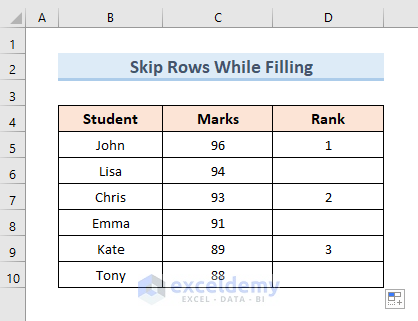
Method 6 – Skip Rows to Fill a Series in Excel
- Select cells D5 and the blank cell D6.
- Drag the Fill Handle tool to cell D10.
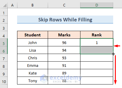
- See that the series is filled by skipping one row.
Method 7 – Fill a Series with Formulas
- Select cell E5. Insert the following formula:
=C5+D5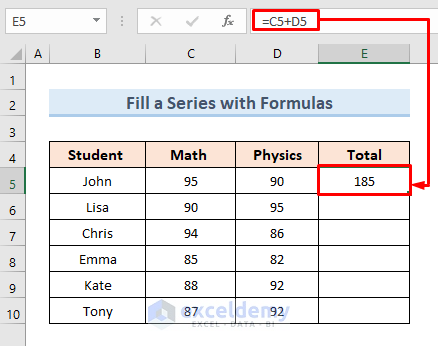
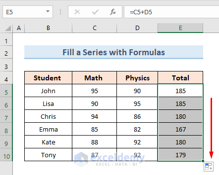
- Drag the Fill Handle tool to cell D10.
- Get the values of totals in series with corresponding formulas.
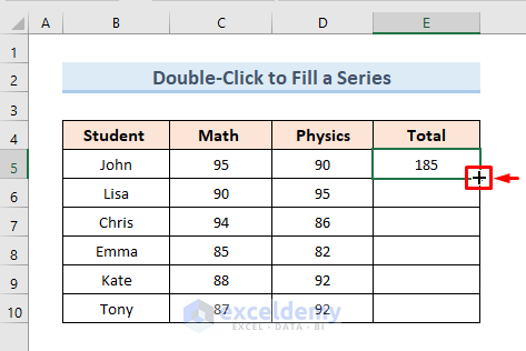
Method 8 – Use of Double-Click to Fill a Series in Excel
- Select cell E5.
- Hover the cursor at the bottom right corner of the cell.
- Double-click on the plus (+).
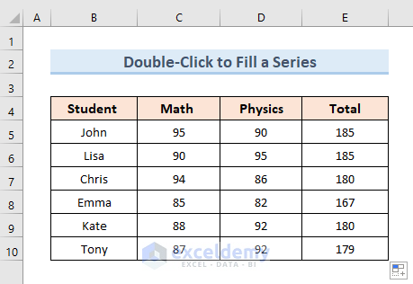
- Get the filled series in the total column.
Method 9 – Excel Filling Days
- Select cell D5.
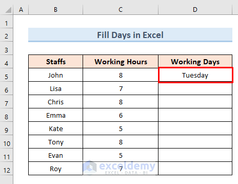
- Drag the Fill Handle tool by using the right-click to cell D12.
- From the available options, select the option Fill Days.
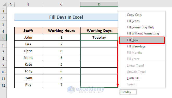
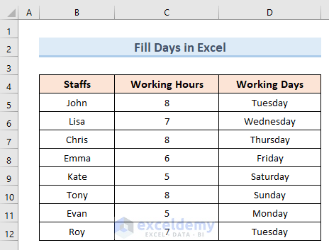
- See the days filled in Column D.
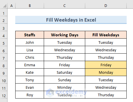
Method 10 – Fill Weekdays in Excel
- Select cell D5.
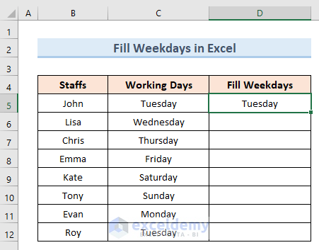
- Drag the Fill Handle tool by using a right-click to cell D12.
- Select the option Fill Weekdays.
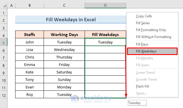
- Get only the weekdays in Column D. We can see that Saturday and Sunday are absent in the series.
Method 11 – Use of Growth Series Option to Fill a Series
11.1 Input Initial Two Numbers in the Growth Series
- Select the given two values.
- Drag the Fill Handle to the bottom by using right-click.
- Select the Growth Trend.
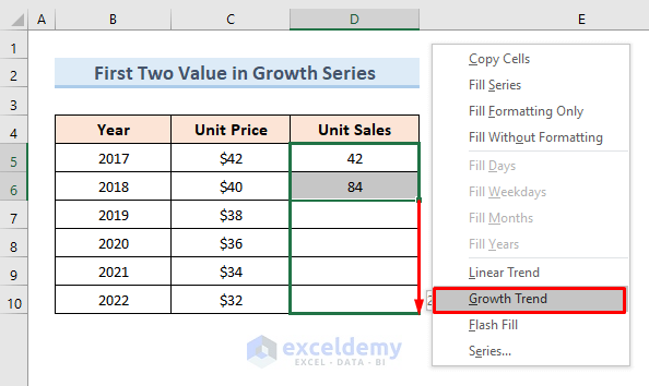
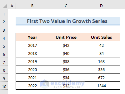
- See that all the values in the Unit Sales column are twice their previous value.
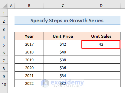
11.2 Specify the Step Value After Inserting First Number in Growth Series
- Select cell D5.
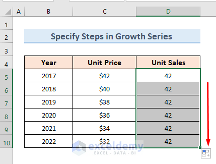
- Drag the Fill Handle tool to cell D10.
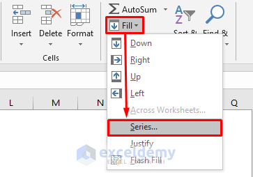
- Go to the Fill option in the editing section of the ribbon.
- Select the option Series.
- A new dialogue box will open. Check the following options:
Type: Growth
Step value: 2
- Press OK.
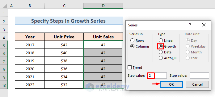
- Get the value of Unit Sales in a series.

Method 12 – Use of Custom Items
12.1 By Using New List of Items
- Go to the File.
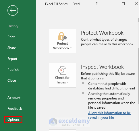
- Select Options.
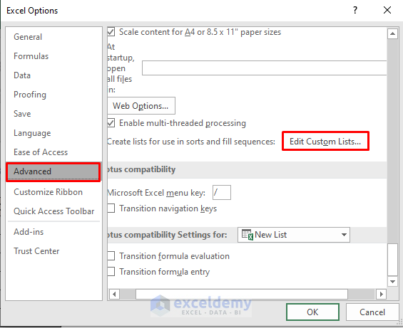
- Go to the Advanced option. Select the option Edit Custom Lists.
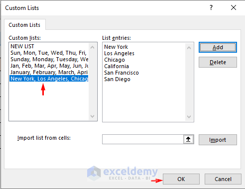
- A new dialogue box named Custom Lists will open.
- Enter the name of the cities in List Entries.
- Click on the option Add.
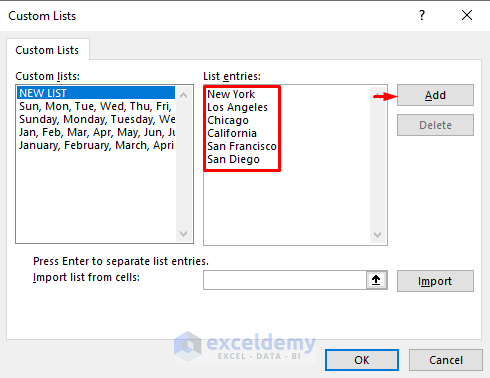
- We get a new list in the Custom List
- Press OK.
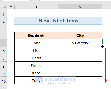
- Insert the first value of the list in cell D5.
- Drag the Fill Handle tool to cell D10.
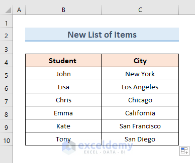
- See the whole list of cities copied in Column C.
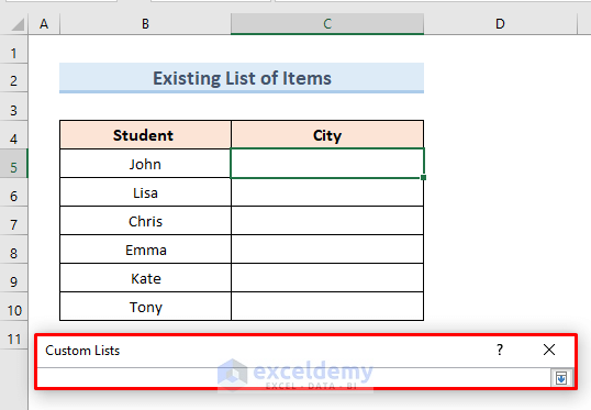
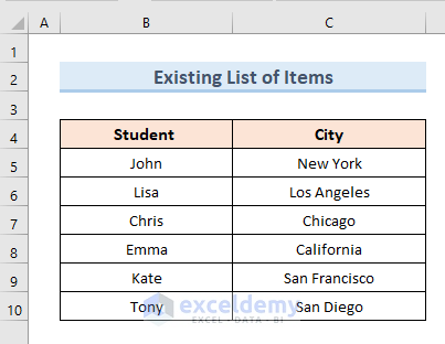
12.2 Based on Existing Items
- Go to the Custom Lists dialogue box.
- Select the import list option.
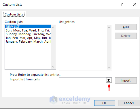
- A new box of commands will open.
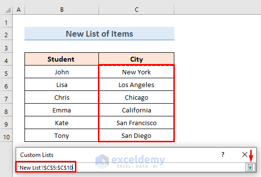
- Go to the previous sheet.
- Select cells C5 to C10.
- Click on the insert option.
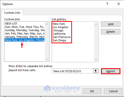
- Hit on the Import.
- We can see our previous list in the Custom lists.
- Enter the first value of the list manually in cell C5.
- Drag the Fill Handle tool to cell C10.
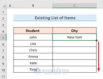
- Get our previous custom list of cities in our new column of cities.
Download Practice Workbook
Download the practice workbook from here.
Related Articles
- How to Create Automatic Rolling Months in Excel
- How to Increment Month by 1 in Excel
- How to Enter Sequential Dates Across Multiple Sheets in Excel
- How to Fill Down Blanks in Excel
- How to Add Sequence Number by Group in Excel
<< Go Back to Excel Autofill | Learn Excel
Get FREE Advanced Excel Exercises with Solutions!

HI,
hiw do i fill series the middle number
i.e.
Unit-305/001/2023
Unit-305/002/2023
Hello Orly, to fill series with the middle number, you should use a formula. In A1 cell, keep the initial value. Then go to A2 cell >> use this formula–> =”Unit-305/”&TEXT(1+ROWS($A$1:A1),”000″)&”/2023″ >> press Enter. After that, drag the Fill Handle icon up to the last cell.
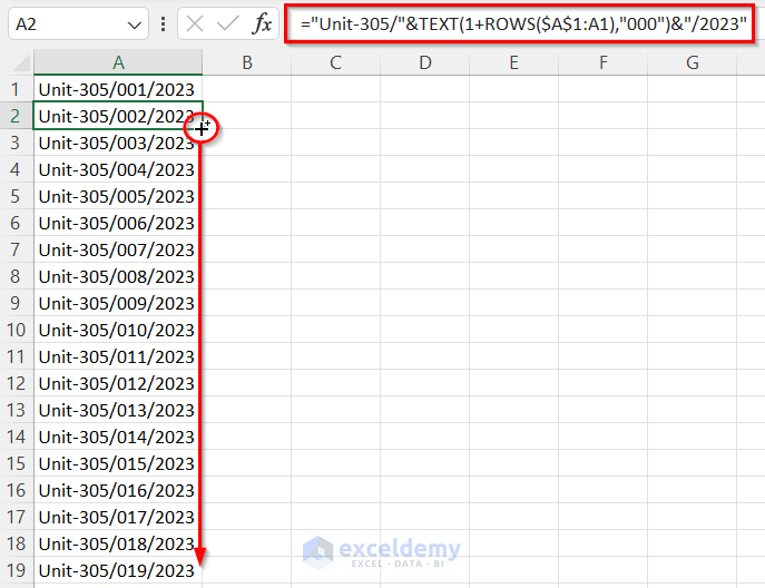
Formula Breakdown
After Equal Sign, write the first fixed part of your value within an Inverted Comma (“Unit-305/”). Then, use Ampersand Operator to join the formula. Here, inside the TEXT function use summation for the increment of middle number. Also, the TEXT function will consider the mentioned pattern (“001”).
Now, again give the Ampersand Operator, and within another Inverted Comma keep the last part of the value (“/2023”).
Regards
Musiha|Exceldemy