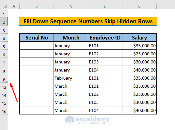
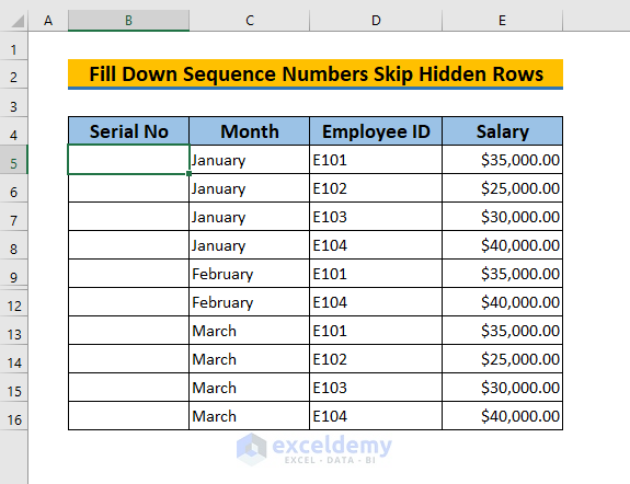
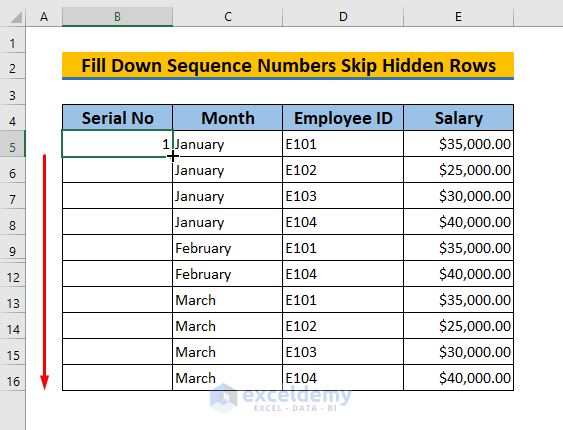
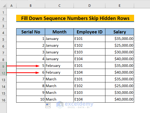
The dataset showcases Serial No, Month, Employee ID, and Salary. Rows 10, 11 and 12 are missing. To fill the sequence in column B skipping hidden rows:
Method 1 – Using the AGGREGATE Function to Fill Sequence Numbers Skipping Hidden Rows in Excel
STEPS:
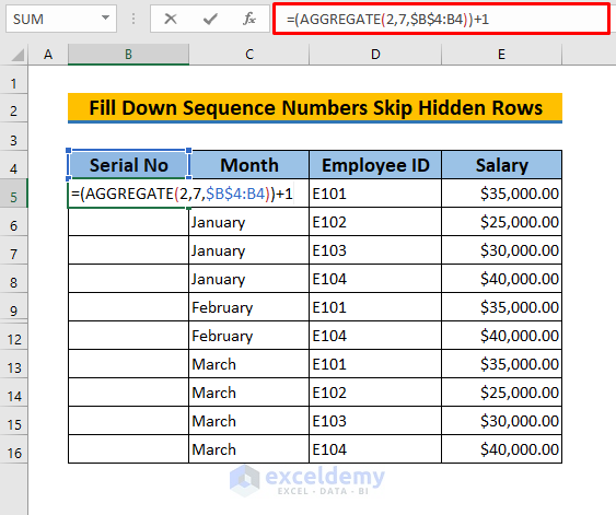
- Select B5
- Enter the following formula:
=(AGGREGATE(2,7,$B$4:B4))+1Formula Breakdown
2 and 7 in (AGGREGATE(2,7,..) represent the nested SUBTOTAL and AGGREGATE function ignoring the hidden rows and error values in $B$4:B4. 1 is added to start the sequence numbers.
- Press ENTER.
You will see 1 in B5.
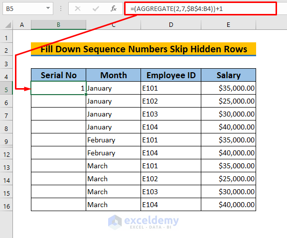
- Drag down the Fill Handle to see the result in the rest of the cells.
This is the output.

Read More: How to Fill Down to Last Row with Data in Excel
2. Fill Down Sequence Numbers Skip Hidden Rows in Excel Using SUBTOTAL Function
STEPS:
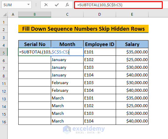
- Select B5.

- Enter the following formula:
=SUBTOTAL(103,$C$5:C5)SUBTOTAL(103,$C$5:C5) represents the total numeric value in $C$5:C5. The first argument 103 refers to the COUNTA function: it counts numbers ignoring the hidden rows and error values.
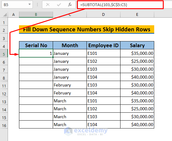
- Press ENTER.
You will see 1 in B5.
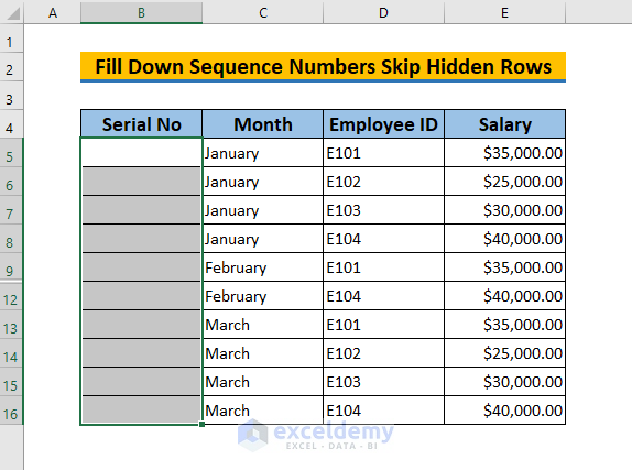
- Drag down the Fill Handle to see the result in the rest of the cells.

This is the output.

Read more: Filling a Certain Number of Rows in Excel Automatically
Method 3 – Using a VBA Code to Fill a Sequence of Numbers Skipping Hidden Rows
STEPS:
- Select B5:B16.
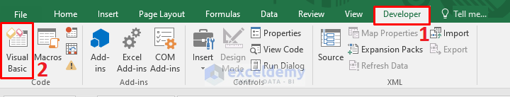
- Go to the Developer Tab >> Select Visual Basic
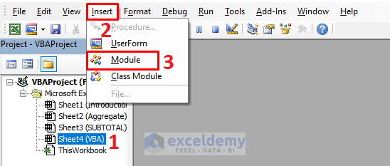
- Select Sheet4 (VBA) >> Go to Insert >> Select Module
- Enter the code in the Module.
Sub FillDownSequenceNumbers()
    Dim Xrng As Range
    Dim Ycell As Range
    Dim ExcelTxt As String
    Dim Xvl As Long
    Dim I As Long
    On Error Resume Next
    ExcelTxt = ActiveWindow.RangeSelection.Address
    Set Xrng = Application.InputBox("Select Range", "Fill Down Sequence Numbers", ExcelTxt, , , , , 8)
    Set Xrng = Xrng.SpecialCells(xlVisible)
    Debug.Print Xrng.Address
    If Xrng Is Nothing Then Exit Sub
    For Each Ycell In Xrng
        Xvl = Xvl + 1
        Ycell = Xvl
    Next
End Sub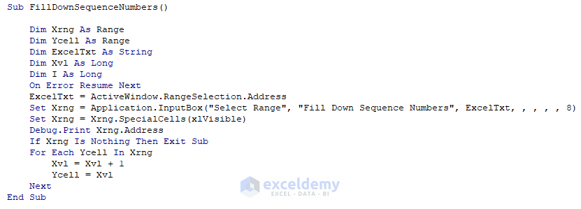
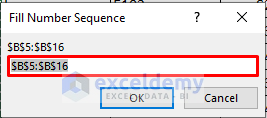
- Press F5 to run the code. In the InputBox , click OK.
This is the output.
Read More: How to Autofill Dates in Excel
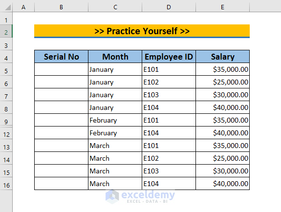
Practice Yourself
Practice here.
Download Practice WorkBook
Related Articles
- How to AutoFill Formula When Inserting Rows in Excel
- How to Fill Column in Excel with Same Value
- How to Autofill a Column in Excel
- How to Auto Populate from Another Worksheet in Excel
<< Go Back to Autofill Numbers | Excel Autofill | Learn Excel
Get FREE Advanced Excel Exercises with Solutions!

When I enter the aggregate the fill handle doesn’t work!
Hello WILL,
Thanks for your feedback. There are some reasons that are why you may have faced the problem. You can solve it by following the steps:
1. Maybe your Fill Handle tool is deactivated. To activate it, Click File > Options > Advanced > Enable fill handle and cell drag and drop.
2. The AGGREGATE function can work only for vertical ranges, not for horizontal ranges. So always apply it for vertical ranges and then the Fill Handle should work.
3. The AGGREGATE function is available since 2010, so if you are using an older version of Excel then it won’t work.
If the above solutions fail to rescue you then your issue is quite particular and that is difficult to find out without the file. So if you share your file with us then we hope, we could provide you with the exact solution.
*Sharing Email Address: [email protected]
I have chosen the SUBTOTAL formula like this
=SUBTOTAL(103,$B$23:B23)*10 because I wanted it to be 10,20,30…..
and it worked for me great.
thanks
Hello Shaul Bel,
Thanks for your appreciation. You’re welcome and I’m really glad to hear that the SUBTOTAL formula worked well for you in achieving the desired results. If you have any more questions or need further assistance with formulas or anything else, feel free to ask!
Regards
ExcelDemy