How to Auto Populate from Another Worksheet in Excel

Method 1 – Linking Excel Worksheets to Auto Populate from Another Worksheet

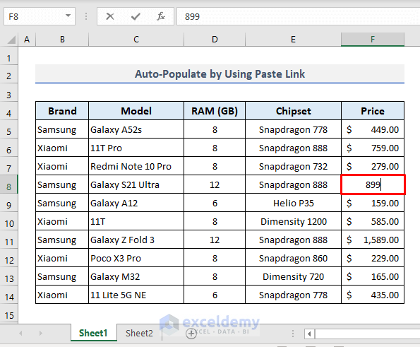
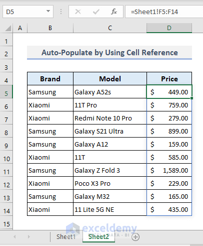
Sheet1 contains some specifications of smartphone models.

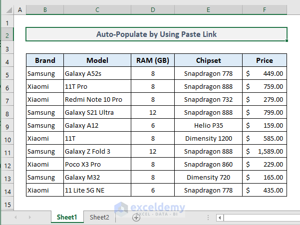
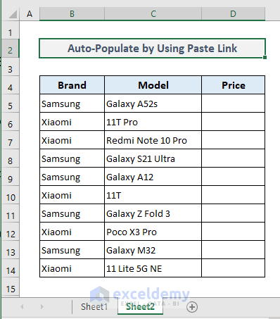
Auto Populate by Linking Worksheets in Excel

In Sheet2, only three columns from the first sheet have been extracted. We’ll show different methods to pull out the price list from the first sheet. We will auto-update the price column if any change is made in the corresponding column in the first sheet (Sheet1).

Auto Populate by Linking Worksheets in Excel

Steps:

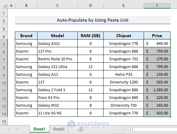
From Sheet1, select the range of cells (F5:F14) containing the prices of the smartphones.
Press Ctrl + C to copy the selected range of cells.

Auto Populate by Linking Worksheets in Excel

Go to Sheet2.
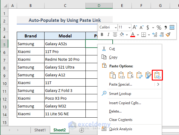
Select the first output cell in the Price column.
Right-click and choose the Paste Link option (the clipboard with a link icon).

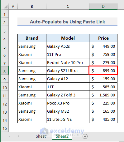
Auto Populate by Linking Worksheets in Excel

The Price column is now complete with the extracted data from the first sheet (Sheet1).
In Sheet1, change the price of any smartphone model.
Press Enter and go to Sheet2.

Auto Populate by Linking Worksheets in Excel

You’ll find the updated price of the corresponding smartphone in Sheet2.

Auto Populate by Linking Worksheets in Excel

You must keep the order of the devices in both sheets the same as this function blindly copies the range without looking at whether other corresponding values match.

Method 2 – Updating Data Automatically by Using the Equal Sign to Refer to Cells from Another Worksheet

Steps:

In Sheet2, select Cell D5 and put an Equal (=) sign.

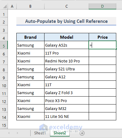
Auto Update Data by Using Equal Sign to Refer Cell(s) from Another Worksheet

Go to Sheet1.
Select the range of cells (F5:F13) containing the prices of all smartphone models.
Press Enter.

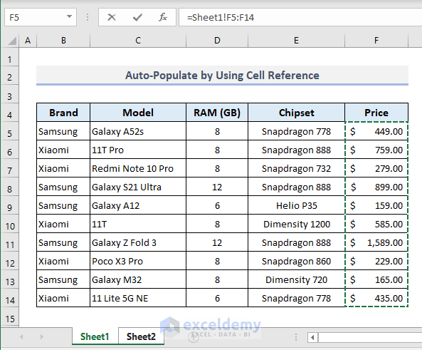
Auto Update Data by Using Equal Sign to Refer Cell(s) from Another Worksheet

In Sheet2, you’ll find an array of prices in Column D ranging from D5 to D14. If you change any data in the Price column in Sheet1, you’ll also see the updated price of the corresponding item in Sheet2 right away.

Auto Update Data by Using Equal Sign to Refer Cell(s) from Another Worksheet

You must keep the order of the devices in both sheets the same as this function blindly copies the range without looking at whether other corresponding values match.

Read More: How to Autofill a Column in Excel

Method 3 – Using an INDEX-MATCH Formula to Auto Populate from Another Worksheet in Excel

Steps:

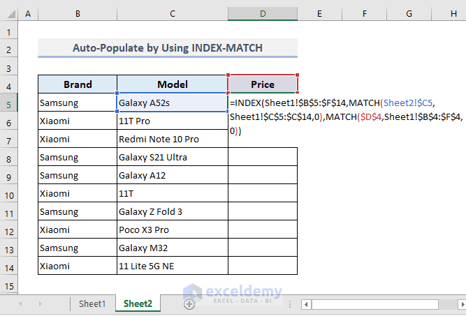
Select Cell D5 in Sheet2 and insert the following formula:

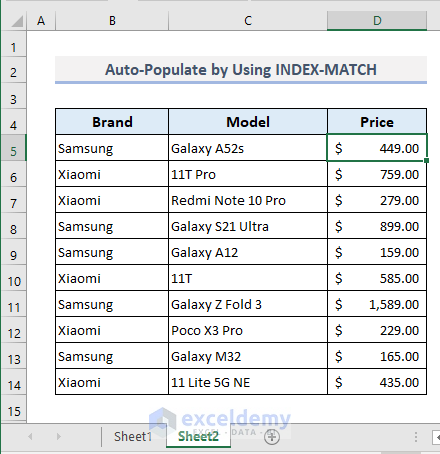
=INDEX(Sheet1!$B$5:$F$14,MATCH(Sheet2!$C35,Sheet1!$C$5:$C$14,0),MATCH($D$4,Sheet1!$B$4:$F$4,0))

Press Enter and you’ll get the first extracted price of the smartphone from Sheet1.

Use of INDEX-MATCH Formula to Auto Populate from Another Worksheet in Excel

Use the Fill Handle to autofill the rest of the cells in Column D.

Use of INDEX-MATCH Formula to Auto Populate from Another Worksheet in Excel

Download the Practice Workbook

Auto Populate from Another Worksheet.xlsx

<< Go Back to Excel Autofill | Learn Excel

Get FREE Advanced Excel Exercises with Solutions!

Sub MoveData() Dim wsSource As Worksheet Dim wsTarget As Worksheet Dim lastRow As Long Set wsSource = ThisWorkbook.Sheets("Source") 'Change to your source sheet name Set wsTarget = ThisWorkbook.Sheets("Target") 'Change to your target sheet name lastRow = wsSource.Cells(wsSource.Rows.Count, "A").End(xlUp).Row wsSource.Rows("1:" & lastRow).Copy wsTarget.Cells(wsTarget.Rows.Count, "A").End(xlUp).Offset(1, 0).PasteSpecial Paste:=xlPasteValues wsSource.Rows("1:" & lastRow).ClearContents End Sub

Sub SyncRowsBasedOnDate() Dim wsMaster As Worksheet, wsWithDate As Worksheet, wsNoDate As Worksheet Dim lastRow As Long, destRowWithDate As Long, destRowNoDate As Long Dim i As Long Dim dateCol As Long Set wsMaster = ThisWorkbook.Sheets("Sheet1") ' Master sheet Set wsWithDate = ThisWorkbook.Sheets("Sheet2") ' Rows with date Set wsNoDate = ThisWorkbook.Sheets("Sheet3") ' Rows without date dateCol = 2 ' Column B holds the date (change to your actual date column) ' Clear old data except headers wsWithDate.Rows("2:" & wsWithDate.Rows.Count).ClearContents wsNoDate.Rows("2:" & wsNoDate.Rows.Count).ClearContents lastRow = wsMaster.Cells(wsMaster.Rows.Count, 1).End(xlUp).Row destRowWithDate = 2 destRowNoDate = 2 For i = 2 To lastRow ' Start from row 2 to skip header If IsDate(wsMaster.Cells(i, dateCol).Value) Then wsMaster.Rows(i).Copy wsWithDate.Rows(destRowWithDate) destRowWithDate = destRowWithDate + 1 Else wsMaster.Rows(i).Copy wsNoDate.Rows(destRowNoDate) destRowNoDate = destRowNoDate + 1 End If Next i End Sub

Sub SyncRowsBasedOnMultipleDates() Dim wsMaster As Worksheet, wsWithDate As Worksheet, wsNoDate As Worksheet Dim lastRow As Long, destRowWithDate As Long, destRowNoDate As Long Dim i As Long, j As Long Dim hasDate As Boolean Dim dateCols As Variant Set wsMaster = ThisWorkbook.Sheets("Sheet1") Set wsWithDate = ThisWorkbook.Sheets("Sheet2") Set wsNoDate = ThisWorkbook.Sheets("Sheet3") ' List all columns with possible dates (for example: columns B to G = 2 to 7) dateCols = Array(2, 3, 4, 5, 6, 7) wsWithDate.Rows("2:" & wsWithDate.Rows.Count).ClearContents wsNoDate.Rows("2:" & wsNoDate.Rows.Count).ClearContents lastRow = wsMaster.Cells(wsMaster.Rows.Count, 1).End(xlUp).Row destRowWithDate = 2 destRowNoDate = 2 For i = 2 To lastRow hasDate = False For j = LBound(dateCols) To UBound(dateCols) If IsDate(wsMaster.Cells(i, dateCols(j)).Value) Then hasDate = True Exit For End If Next j If hasDate Then wsMaster.Rows(i).Copy wsWithDate.Rows(destRowWithDate) destRowWithDate = destRowWithDate + 1 Else wsMaster.Rows(i).Copy wsNoDate.Rows(destRowNoDate) destRowNoDate = destRowNoDate + 1 End If Next i End Sub

Private Sub Worksheet_Change(ByVal Target As Range) ' === Settings: change to match your file === Const URL_CELL As String = "B3" ' URL input cell on Sheet1 Const LOG_SHEET_NAME As String = "Sheet2" ' Sheet that stores the log Const QR_SHAPE_NAME As String = "" ' Optional: name of QR image on Sheet1 (leave "" if unknown) On Error GoTo Done If Intersect(Target, Me.Range(URL_CELL)) Is Nothing Then Exit Sub Application.EnableEvents = False Dim urlVal As String urlVal = Trim$(Me.Range(URL_CELL).Value) If Len(urlVal) = 0 Then GoTo Done ' ignore blanks Dim wsLog As Worksheet Set wsLog = ThisWorkbook.Worksheets(LOG_SHEET_NAME) ' Next empty row (keeps row 1 for headers) Dim r As Long r = wsLog.Cells(wsLog.Rows.Count, "A").End(xlUp).Row + 1 If r < 2 Then r = 2 ' Log timestamp + URL wsLog.Cells(r, "A").Value = Now wsLog.Cells(r, "B").Value = urlVal ' --- Copy QR image from Sheet1 to Sheet2 (column C) --- Dim src As Shape Set src = Nothing ' Try by given name first If Len(QR_SHAPE_NAME) > 0 Then On Error Resume Next Set src = Me.Shapes(QR_SHAPE_NAME) On Error GoTo 0 End If ' If not found, pick the largest picture on Sheet1 If src Is Nothing Then Dim shp As Shape, biggest As Double For Each shp In Me.Shapes If shp.Type = msoPicture Then If shp.Width * shp.Height > biggest Then biggest = shp.Width * shp.Height Set src = shp End If End If Next shp End If ' Paste into Sheet2, column C If Not src Is Nothing Then src.Copy wsLog.Range("C" & r).PasteSpecial ' Format the pasted image (last shape on the sheet) Dim pasted As Shape Set pasted = wsLog.Shapes(wsLog.Shapes.Count) With pasted .LockAspectRatio = msoTrue .Top = wsLog.Cells(r, "C").Top + 2 .Left = wsLog.Cells(r, "C").Left + 2 .Height = wsLog.Rows(r).RowHeight * 1.8 ' adjust size if you want End With End If Done: Application.EnableEvents = True End Sub

30 Comments

Paul R Hartley Feb 18, 2022 at 11:55 PM

I have a “form” (Xcell sheet) that my customer fills out, and then I want to get that data to populate into the cells of my own Xcell workbook. The problem is that if I copy the “Form” into my Workbook, whatever links I had setup previously will not link to the new “Form”…even if I give the Form Tab the same name as the previous one….the links are broken and would have to be re-set.

Do you know a way to allow these links to the new Data to be maintained?

thank you for any ideas you may have!
- Reply
  Tanjim Reza Aug 14, 2022 at 2:52 PM
  
  Hi PAUL R HARTLEY! Thank you for your query.
  
  You can fix these links easily using the following process.
  Go to the Data tab >> Queries & Connections group >> Edit Links tool.
  Afterward, all the links used in this workbook will be shown to you in the Edit Links window. Select individual links and click on the Check Status button for each of them.
  If you see an Error: Source not found in any status, click on the Change Source button. Subsequently, browse your “form” Excel sheet >> click on the OK button >> click on the Close button of the Edit Links window.
  
  Regards,
  Tanjim Reza
ANTHONY Apr 23, 2022 at 6:18 AM

WHEN YOU GO TO PASTE YOU CAN CLICK PASTE SPECIAL AND THEN SCROLL TO THE BOTTOM TO PASTE SPECIAL IT WILL GIVE YOU A MENU TO CHOOSE EXACTLY WHAT YOU NEED PASTED. THERE IS A CHOICE FOR PASTE LINK. YOU CAN TRY THAT
- Reply
  Masum Mahdy Aug 14, 2022 at 9:59 AM
  
  We appreciate your nice suggestion, ANTHONY! You can also see the following article to know about all the Paste Options in Excel.
  https://www.exceldemy.com/paste-options-in-excel/
  
  Thank you for being with us. 🙂
Mrs B Feb 13, 2023 at 11:41 PM

Good day

I have a spreadsheet with employee information that have been awarded bursaries. They’re studying with different universities and these universities have vendor codes. I need to create individual payment requisitions using a template. How do I only change the employee number in the payment requisition and the form auto populates other fields relating to that particular employee?
- Reply
  Sabrina Ayon Feb 14, 2023 at 2:08 PM
  
  Hello, MRS B!
  Can you please send me your excel file via email? ([email protected]), so that I can solve your problem!
  
  Right now I’m giving you a quick solution without the dataset. You can use Excel’s VLOOKUP function to have fields in the payment request form automatically fill in depending on the employee number.
  
  Here is a formula that uses the VLOOKUP function as an example:
  
  =VLOOKUP(employee number,employee table,2,FALSE)
  
  Here, “Employee number” refers to the cell where the employee number input is located, “Employee table” refers to the cell range containing the employee information table, which includes the employee number in the first column, and “2” refers to the column number in the table that contains the university information.
  
  You can change this formula to return different data. Once the relevant information has been obtained from the table, you can use it to fill in the essential fields on the payment request form by utilizing straightforward cell references or other procedures.
  
  Hope this will help you.
  Good Luck!
  
  Regards,
  Sabrina Ayon
  Author, ExcelDemy.
VITO CASA Apr 3, 2024 at 9:39 PM

Good day, Looking for some help.

I have a list of tasks on sheet1 that fall on different dates. I’m for a formula or macro that will extract that info and plan it on sheet2 based on the dates.
- Reply
  Lutfor Rahman Shimanto Apr 4, 2024 at 2:29 PM
  Hello Vito Casa
  
  Thanks for visiting our blog and sharing your questions. Sheet1 contains a list of tasks with corresponding dates. You want to extract this information and plan the tasks on Sheet2 based on the dates. To do so, you can develop multiple formulas using VLOOKUP, INDEX, MATCH, and XLOOKUP. You can also use IFERROR to handle errors.
  
  SOLUTION Overview:
  Using VLOOKUP and IFERROR Functions
  
  Using INDEX, MATCH and IFERROR Functions
  
  Using XLOOKUP Function
  NOTE: If you are a Microsoft 365 user, you will be able to use the XLOOKUP function.
  
  I hope the formulas mentioned will reach your goal. I have attached the solution workbook as well; good luck.
  
  DOWNLOAD SOLUTION WORKBOOK
  
  Regards
  Lutfor Rahman Shimanto
  ExcelDemy
  - Reply
    VITO CASALINUOVO Apr 9, 2024 at 9:42 PM
    
    Thank you, I appreciate your work. I just have one problem. I have multipole task that fall on the same day. Is there a way to capture all
    - Lutfor Rahman Shimanto Apr 16, 2024 at 4:43 PM
      
      Dear Vito Casalinuovo
      
      It is good to see you again. Yes! You can capture all the tasks that fall on the same day. To do so, use the IFERROR, TEXTJOIN and FILTER function:
      
      SOLUTION Overview:
      
      Follow these steps:
      
      Choose cell C3.
      
      Insert the following formula: =IFERROR(TEXTJOIN(", ",TRUE, FILTER(Sheet1!$C$3:$C$7, Sheet1!$B$3:$B$7=Sheet2!$B3)), "")
      
      Drag the Fill Handle icon to copy the formula down.
      
      I hope you have found the formula helpful. I am also attaching the solution workbook; good luck.
      
      DOWNLOAD SOLUTION WORKBOOK
      
      Regards
      Lutfor Rahman Shimanto
      ExcelDemy
VITO CASALINUOVO Apr 8, 2024 at 9:39 PM

That looks great. I only have one issue. the formula doesn’t pick up multiple tasks set for a set date. i.e April 10th I have 3 tasks. Can the formula be adjusted?
- Reply
  Lutfor Rahman Shimanto Apr 17, 2024 at 10:08 AM
  Dear Vito Casalinuovo
  
  Thanks for further clarifying your problem. Based on the requirement, I have come up with another solution, though the previous solution works perfectly on our end.
  
  Assuming you have a dataset like the following:
  
  You want to get all the tasks that fall on the same day. To achieve the goal, you can combine:
  IFERROR, TEXTJOIN and IF Functions (New)
  =IFERROR(TEXTJOIN(", ", TRUE, IF(Sheet1!$B$3:$B$11=Sheet2!$B3, Sheet1!$C$3:$C$11, "")), "")
  
  IFERROR, TEXTJOIN and FILTER Functions (Previous)
  =IFERROR(TEXTJOIN(", ", TRUE, FILTER(Sheet1!$C$3:$C$11, Sheet1!$B$3:$B$11=Sheet2!$B3)), "")
  I hope these formulas will help you to reach your goal. I have attached the solution workbook as well; good luck.
  
  DOWNLOAD SOLUTION WORKBOOK
  
  Regards
  Lutfor Rahman Shimanto
  ExcelDemy
Vito May 3, 2024 at 8:26 PM

Good day, Sorry for the late response. I will give this a try and I will report back.
- Reply
  Shamima Sultana May 5, 2024 at 10:44 AM
  
  Hello Vito,
  
  Don’t be sorry Vito. Let us know your feedback, hopefully it will work.
  
  Regards
  ExcelDemy
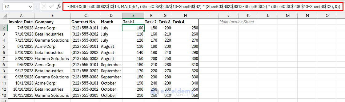
yulissa alvarez Jun 25, 2024 at 4:36 AM

hi folks, i have a pretty big workbook im working on and am looking for a specific formula or way to auto populate one sheet based on information from another. short version is: in sheet b i need a cell to populate from sheet c based on a name, a contract number, a month, and the task (theres 4 tasks), these are on tables, do i need to convert to range instead?

tldr:
i am tracking invoices for the fiscal year of july 23- june 24. there are 13 different companies we work with, and they invoice us monthly based on 3-4 deliverables depending on contract (there’s two contracts). my invoice sheet has all invoices and the deliverables they are charging us for. my other two sheets have deliverables that were reported online and to another funder, i need to make sure they all match but i dont want to hop between sheets, i want my main sheet to populate those numbers and i can create a conditional format after. keep in mind that the other two sheets are in order of month and company, the invoice sheet is in order of when the invoice was received.
- Reply
  Shamima Sultana Jun 25, 2024 at 4:03 PM
  
  Hello Yulissa Alvarez,
  
  Based on your given scenario created a dummy dataset to auto populate one sheet values based on information from another sheet.
  
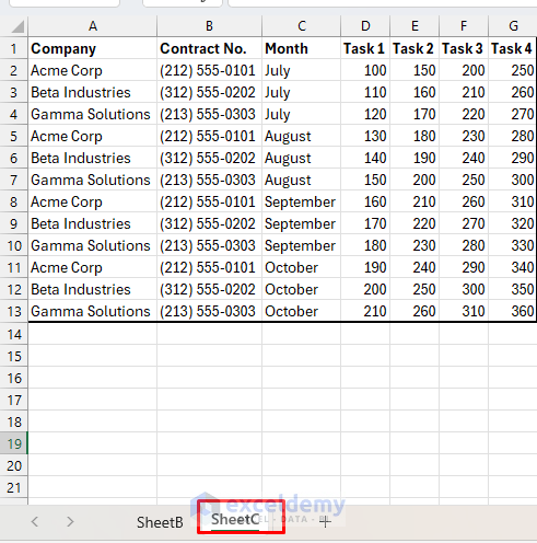
  Here I used INDEX-MATCH functions to get data from another sheet dynamically.
  Use the following formulas:
  Task1: =INDEX(SheetC!$D$2:$D$13, MATCH(1, (SheetC!$A$2:$A$13=SheetB!$B2) * (SheetC!$B$2:$B$13=SheetB!$C2) * (SheetC!$C$2:$C$13=SheetB!$D2), 0))
  Task2: =INDEX(SheetC!$E$2:$E$13, MATCH(1, (SheetC!$A$2:$A$13=SheetB!$B2) * (SheetC!$B$2:$B$13=SheetB!$C2) * (SheetC!$C$2:$C$13=SheetB!$D2), 0))
  Task3: =INDEX(SheetC!$F$2:$F$13, MATCH(1, (SheetC!$A$2:$A$13=SheetB!$B2) * (SheetC!$B$2:$B$13=SheetB!$C2) * (SheetC!$C$2:$C$13=SheetB!$D2), 0))
  Task4: =INDEX(SheetC!$G$2:$G$13, MATCH(1, (SheetC!$A$2:$A$13=SheetB!$B2) * (SheetC!$B$2:$B$13=SheetB!$C2) * (SheetC!$C$2:$C$13=SheetB!$D2), 0))
  
  If you want to add more task just change the cell-refernce.
  Output:
  
  You can Download the Excel file:
  Auto Populate Values from Another Sheet
  
  Regards
  ExcelDemy
Brea Kelley Sep 4, 2024 at 4:54 AM

Hi, Love your site! I hope you can help me come up with a solution. I am trying to auto populate venue prices from one sheet to another sheet but have the appropriate price auto populate based on the data entered in column to the left.

Here’s an example: I am working on sheet titled Events. Column F has the names of the venue for each event. Column G would be where the price goes. All prices for each venue is listed in the sheet title Venue Costs. How can I get column G in the Events sheet to populate the appropriate prices from the Venue Costs sheet but pull the correct price based on the venue listed in Column F?

Is that even possible?
- Reply
  Shamima Sultana Sep 4, 2024 at 8:54 PM
  
  Hello Brea Kelley,
  
  Yes, you can auto populate venue prices in Column G of the Events sheet based on the venue listed in Column F by using the VLOOKUP function.
  
  Use the following formula:
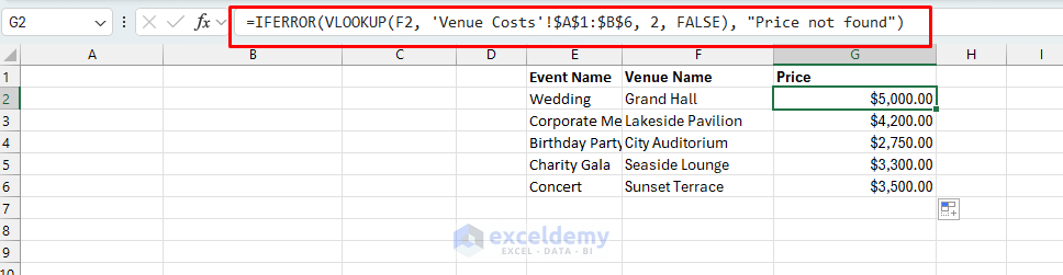
  =IFERROR(VLOOKUP(F2, ‘Venue Costs’!$A$1:$B$6, 2, FALSE), “Price not found”)
  
  Change the cell reference of of Venue Costs sheet based on your data.
  
  Download the Excel file:
  Auto Populate Value from Another Sheet.xlsx
  Regards
  ExcelDemy
  - Reply
    TJ Nov 11, 2024 at 8:27 PM
    
    I have a similar situation, however, mine is about parts lists. Each day, our department head sends us a list of orders to fill. We have a master document that contains a breakdown of each item and the parts used to make the products. Our associates manually search this master document daily to use our inventory platform to know how many smaller parts need to be ordered to fulfill the daily orders. I feel like this formula will also work for my specific situation, however, our master document list contains multiple rows of items for the breakdown of parts per item. Is there a way to input the daily list onto a workbook and have Excel input new rows under each item with the detailed breakdown of the parts needed?
    - Shamima Sultana Nov 12, 2024 at 9:57 AM
      
      Hello TJ,
      
      Yes, there is a way to automate your parts breakdown in Excel by using a combination of formulas.
      
      If your master document has a detailed breakdown of parts for each item, and you want to pull this breakdown dynamically into your daily order list, here’s a simple approach using the FILTER function (available in Excel 365 and Excel 2019) or the VLOOKUP function combined with helper columns.
      
      If your breakdown list is well-structured, the FILTER function can pull in all matching parts for a given item. In a cell where you want the parts listed, you can use:
      
      =FILTER(Master!B2:D100, Master!A2:A100 = OrderList!A2, “No parts found”)
      
      Replace Master!B2:D100 with the range containing your parts details, and Master!A2:A100 with the range containing item names in your master list. OrderList!A2 would be the item name in your daily order sheet.
      
      Let me know if you’d like more detailed steps on any of these methods!
      
      Best Regards,
      ExcelDemy
Josi Dec 5, 2024 at 2:48 AM

Hello everyone. I’m hoping to auto move data from one sheet to the other, then have the previous data auto delete without deleting on the new sheet. Is this possible?
- Reply
  Shamima Sultana Dec 5, 2024 at 10:41 AM
  Hello Josi,
  
  Yes, it is possible to move data from one sheet to another automatically while retaining the original data in the new sheet. This can be done using VBA (Visual Basic for Applications) to automate the process. The script can copy data to the target sheet and clear the original while keeping the target data intact.
  
  Here’s a VBA script to automate this process:
  
  1. Press Alt + F11 to open the VBA editor.
  2. Insert a Module and paste the following code:
```
Sub MoveData()
    Dim wsSource As Worksheet
    Dim wsTarget As Worksheet
    Dim lastRow As Long
    
    Set wsSource = ThisWorkbook.Sheets("Source") 'Change to your source sheet name
    Set wsTarget = ThisWorkbook.Sheets("Target") 'Change to your target sheet name
    
    lastRow = wsSource.Cells(wsSource.Rows.Count, "A").End(xlUp).Row
    wsSource.Rows("1:" & lastRow).Copy
    wsTarget.Cells(wsTarget.Rows.Count, "A").End(xlUp).Offset(1, 0).PasteSpecial Paste:=xlPasteValues
    wsSource.Rows("1:" & lastRow).ClearContents
End Sub
```
  3. Run the Macro to transfer and clear the source data.
  
  Regards
  ExcelDemy
Ryan Jul 10, 2025 at 11:15 PM

Hi,

I’m Trying to populate two separate sheets with data from a main master sheet. I’ve created similar tables with identical formatting across all three sheets. what I’d like to happen is if you input a date into one of the cells on the master table on sheet 1 it copies that row to the table on sheet 2 but if no dates exist within that row on sheet one then that row is copied to sheet 3. Also, if there was a date on sheet 1 but that date is removed from sheet 1 that row is removed form sheet 2 and added to sheet 3 and vice versa.
- Reply
  Shamima Sultana Jul 11, 2025 at 10:50 AM
  Hello Ryan,
  
  Great question! What you’re describing is possible in Excel, but it usually requires a combination of formulas or VBA (macros), since you want the data on Sheet 2 and Sheet 3 to automatically update based on whether there is a date in the row on your master sheet (Sheet 1).
  
  Use Formulas (For Viewing Only, Not for Actual Row Copy)
  If you just want to display rows from the master sheet on Sheet 2 and Sheet 3 (without actually copying and removing rows), you can use formulas like FILTER (in Excel 365/2021), or helper columns with IF and INDEX/MATCH in older versions.
  
  For Sheet 2 (rows with dates):
  =FILTER(‘Sheet1’!A2:D100, ISNUMBER(‘Sheet1’!B2:B100))
  (Assuming the date is in column B. Adjust range as needed.)
  
  For Sheet 3 (rows without dates):
  =FILTER(‘Sheet1’!A2:D100, NOT(ISNUMBER(‘Sheet1’!B2:B100)))
  
  VBA Approach
  This VBA solution will copy (not move) the relevant rows to Sheet2 and Sheet3 each time you make a change in the Master sheet. Sheet2 and Sheet3 are refreshed every time, so they always show the correct filtered rows.
  1. Press ALT + F11 to open the VBA editor.
  2. Insert a new module (Right-click on any object in the Project Explorer > Insert > Module).
  3. Copy and paste the following code into the module.
```
Sub SyncRowsBasedOnDate()
    Dim wsMaster As Worksheet, wsWithDate As Worksheet, wsNoDate As Worksheet
    Dim lastRow As Long, destRowWithDate As Long, destRowNoDate As Long
    Dim i As Long
    Dim dateCol As Long
    
    Set wsMaster = ThisWorkbook.Sheets("Sheet1")      ' Master sheet
    Set wsWithDate = ThisWorkbook.Sheets("Sheet2")    ' Rows with date
    Set wsNoDate = ThisWorkbook.Sheets("Sheet3")      ' Rows without date
    
    dateCol = 2  ' Column B holds the date (change to your actual date column)
    
    ' Clear old data except headers
    wsWithDate.Rows("2:" & wsWithDate.Rows.Count).ClearContents
    wsNoDate.Rows("2:" & wsNoDate.Rows.Count).ClearContents
    
    lastRow = wsMaster.Cells(wsMaster.Rows.Count, 1).End(xlUp).Row
    
    destRowWithDate = 2
    destRowNoDate = 2
    
    For i = 2 To lastRow   ' Start from row 2 to skip header
        If IsDate(wsMaster.Cells(i, dateCol).Value) Then
            wsMaster.Rows(i).Copy wsWithDate.Rows(destRowWithDate)
            destRowWithDate = destRowWithDate + 1
        Else
            wsMaster.Rows(i).Copy wsNoDate.Rows(destRowNoDate)
            destRowNoDate = destRowNoDate + 1
        End If
    Next i
End Sub
```
  Auto-Run Macro When Master Sheet Changes
  To make the macro run automatically when you change anything in the master sheet:
  1. In the VBA editor, double-click on Sheet1 (or your master sheet).
  2. Paste this code:
```
Private Sub Worksheet_Change(ByVal Target As Range)
    Application.EnableEvents = False
    SyncRowsBasedOnDate
    Application.EnableEvents = True
End Sub
```
  Regards
  ExcelDemy
  - Reply
    Ryan Jul 17, 2025 at 5:25 AM
    
    Fantastic!! One last issue the lines that you instructed me to put in to have the macro run automatically aren’t working. I still have to click run for the macro to populate everything.
    - Shamima Sultana Jul 19, 2025 at 11:48 AM
      
      Hello Ryan,
      
      Thank you for your feedback! If the macro isn’t running automatically, you’ll want to use a worksheet or workbook event to trigger it. For example, you can place the macro call inside the Worksheet_Change event (for changes in a specific sheet) or in the Workbook_Open event (to run when the file opens).
      
      Example (run automatically when data changes in Sheet1):
      
      1. Right-click the Sheet1 tab and choose View Code.
      2. Paste this code in the code window:
      
      Private Sub Worksheet_Change(ByVal Target As Range)
      Call SyncRowsBasedOnMultipleDates
      End Sub
      
      Now, whenever you change any data in Sheet1, the macro will run automatically.
      
      Regards
      ExcelDemy
  - Reply
    Ryan Jul 11, 2025 at 8:27 PM
    
    This is awesome thank you. How would this change if I had multiple columns that could have dates in them (I currently have 6)
    - Shamima Sultana Jul 12, 2025 at 12:09 PM
      
      Hello Ryan,
      
      Thank you so much for your feedback! If you have multiple columns that could contain dates (for example, 6 different columns), you just need to adjust the VBA code so that it checks all those columns in each row. If any of those columns has a date, the row will go to Sheet2; if none have dates, the row will go to Sheet3.
      
      Here’s how you can update the macro:
      
      Sub SyncRowsBasedOnMultipleDates() Dim wsMaster As Worksheet, wsWithDate As Worksheet, wsNoDate As Worksheet Dim lastRow As Long, destRowWithDate As Long, destRowNoDate As Long Dim i As Long, j As Long Dim hasDate As Boolean Dim dateCols As Variant Set wsMaster = ThisWorkbook.Sheets("Sheet1") Set wsWithDate = ThisWorkbook.Sheets("Sheet2") Set wsNoDate = ThisWorkbook.Sheets("Sheet3") ' List all columns with possible dates (for example: columns B to G = 2 to 7) dateCols = Array(2, 3, 4, 5, 6, 7) wsWithDate.Rows("2:" & wsWithDate.Rows.Count).ClearContents wsNoDate.Rows("2:" & wsNoDate.Rows.Count).ClearContents lastRow = wsMaster.Cells(wsMaster.Rows.Count, 1).End(xlUp).Row destRowWithDate = 2 destRowNoDate = 2 For i = 2 To lastRow hasDate = False For j = LBound(dateCols) To UBound(dateCols) If IsDate(wsMaster.Cells(i, dateCols(j)).Value) Then hasDate = True Exit For End If Next j If hasDate Then wsMaster.Rows(i).Copy wsWithDate.Rows(destRowWithDate) destRowWithDate = destRowWithDate + 1 Else wsMaster.Rows(i).Copy wsNoDate.Rows(destRowNoDate) destRowNoDate = destRowNoDate + 1 End If Next i End Sub
      
      Just update the dateCols array to match the columns you’re using for dates.
      Let me know if you need help customizing this further!
      
      Regards
      ExcelDemy

matmat Sep 5, 2025 at 1:37 PM

Hi, I have a question. I’m working with the QRCode generator template in excel. What I want, is, each time I change the cell containing the url in sheet 1 (the qr code generator template), it fills automaticaly a new cell in sheet 2. The goal here is to maintain a listing of all urls generated..And if it’s possible also, each time the image of the qr code changes in sheet 1, auto fill a second cell in sheet 2…Is this even possible ? I read maybe all the tutorial here and others website, I don’t find a similar example.

Shamima Sultana Sep 8, 2025 at 10:29 AM

Hello Matmat,

Yes, it’s possible, but not with normal Excel formulas. You’ll need a small VBA macro. The idea is:

1. Every time you type a new URL in Sheet1, the macro will copy that URL into the next empty row on Sheet2.
2. At the same time, it can also copy the QR code image from Sheet1 and paste it beside the URL in Sheet2.

This way you’ll build a full list of URLs and their QR codes automatically.

Paste the code into the Sheet1 code window.

Change these to match your file:
1. URL_CELL → the cell where you type the URL on Sheet1 (example: “B3”).
2. LOG_SHEET_NAME → your log sheet name (example: “Sheet2”).
3. QR_SHAPE_NAME → the exact name of the QR picture on Sheet1 (leave as “” if unknown).
4. In Sheet2, put headers: A1=Timestamp, B1=URL, C1=QR Image.

Regards,
ExcelDemy

How to Auto Populate from Another Worksheet in Excel

Method 1 – Linking Excel Worksheets to Auto Populate from Another Worksheet

Method 2 – Updating Data Automatically by Using the Equal Sign to Refer to Cells from Another Worksheet

Method 3 – Using an INDEX-MATCH Formula to Auto Populate from Another Worksheet in Excel

Related Articles

Leave a reply Cancel reply