Method 1 – Using the Fill Series Option to Autofill Numbers
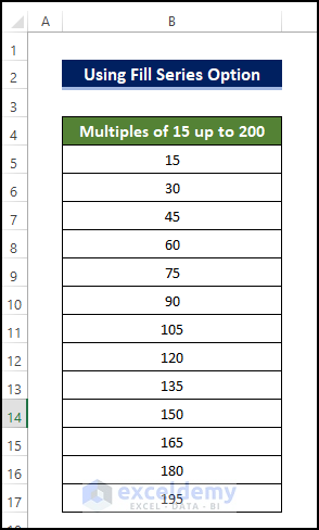
We’re going to create a series of numbers in multiples of 15, up to 200.
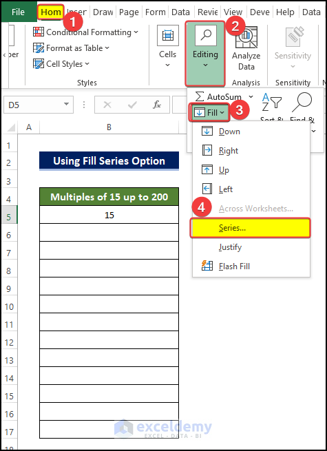
Steps:
- Go to the Home tab.
- Go to the Editing group of commands.
- Click on the Fill drop-down.
- Select Series.
- You’ll get a box with multiple options to choose from.
- Insert 15 as Step Value.
- Type 200 inside Stop Value.
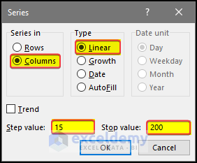
- Click OK and you’ll get the list of numbers, up to 195 (as it’s the last multiple of 15 that is under 200).
Read More: Drag Number Increase Not Working in Excel
Method 2 – Using Flash Fill to Autofill Numbers
We have a list of names and ID numbers of some students in a school. We only need their ID numbers.
Steps:
- Type the first ID number from Cell B4 in the column of ID (Column C) in cell C4.
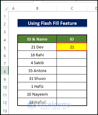
- Select the Fill drop-down under the Home tab.
- Click on the Flash Fill command.
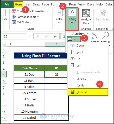
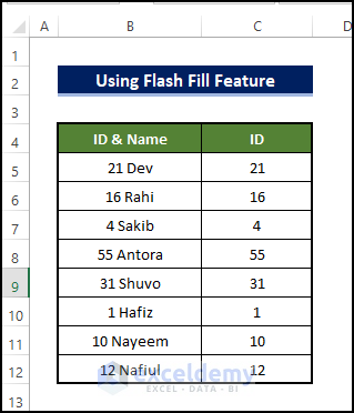
- The ID numbers of all students in your list will be displayed.
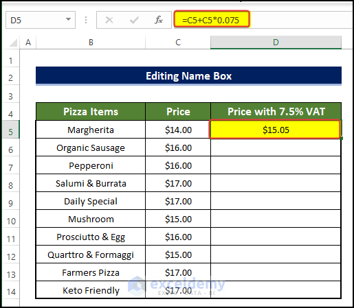
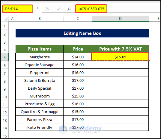
Method 3 – Editing the Name Box to Autofill Numbers in Excel
We have a list of pizza prices and want to calculate the final prices with 7.5% VAT.
Steps:
- Multiply C5 with 1.075 (for 7.5% VAT, the multiplier will be 1.075) at Cell D5.
- You’ll get the price including VAT for the item Margherita.
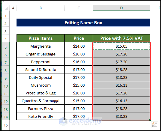
- Copy D5.
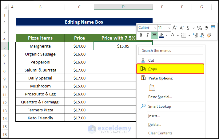
- Go to the Name Box and input your cell range D5:D14 for calculation.
- Press Enter.
- Press Ctrl + V.
- You’ll get all the final prices including VAT for all pizzas under Column D.
Method 4 – Copying Formula(s) and Then Navigating to Paste to Autofill Numbers
Steps:
- Calculate the final price at D5 for the first value as in Method 3.
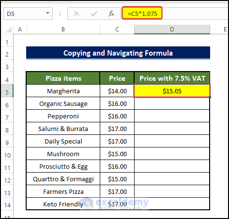
- Copy D5.
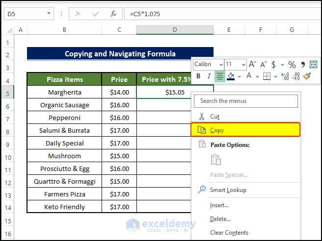
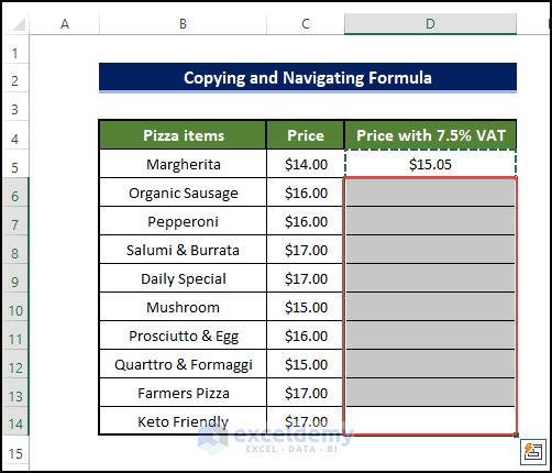
- Navigate to C2 by pressing the Left Arrow key.
- Press Ctrl + Down Arrow to reach the last cell (C14) in column C.
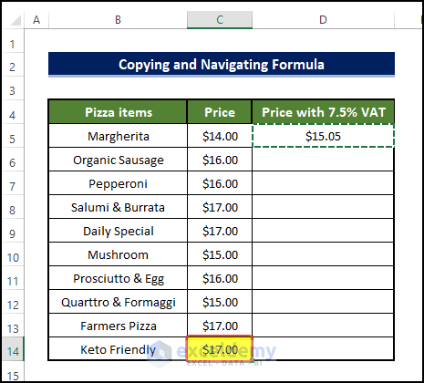
- Navigate to D14 with the Right Arrow key and press Ctrl + Shift + Up Arrow.
- It’ll select the whole column range (D2:D14) where you need the overall calculated results.
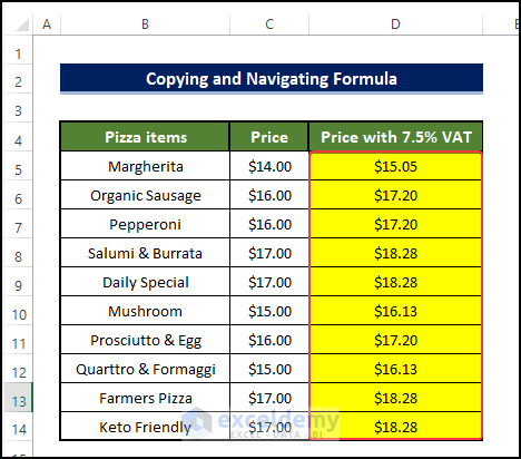
- Press Ctrl +V to paste, and you’ll find your desired results in column D.
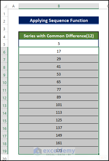
Method 5 – Applying the SEQUENCE Function to Autofill Numbers
We want a series starting from 5 and with a step of 12. Let’s get a list of the first 15 numbers.
Steps:
- In the Function Bar, insert:
=SEQUENCE(15, 1, 5, 12)15 denotes the number of rows you want to see, while 1 is for column numbers the sequence will use (i.e., the range will take 15 cells in a single column). 5 is the initial value you want to start from, and 12 is for the step value.
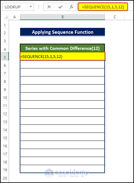
- Press Enter and you’ll get the full series.
Read More: How to Auto Number Cells in Excel
How to Autofill Formula in Excel Without Dragging
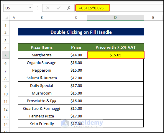
Method 1 – Double-Clicking on the Fill Handle
Steps
- We need to calculate the Price with 7.5% VAT of the product mentioned in the range of cells B5:B14.
- Select cell D5 and enter the following formula:
=C5+C5*0.075
- Hover over the Fill Handle icon in the bottom-right corner of cell D5.
- Double-click on the Fill Handle.
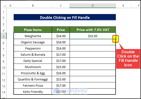
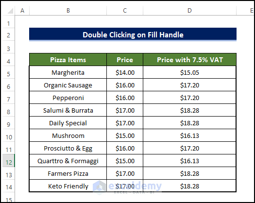
- The range of cells D5:D14 is now filled with the price value with a 7.5% increase.
Method 2 – Using a Keyboard Shortcut to Fill Adjacent Cells with Formulas
Steps
- We need to calculate the Price with 7.5% VAT of the product mentioned in the range of cells B5:B14.
- Select cell D5 and enter the following formula:
=C5+C5*0.075
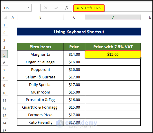
- Select the range of cells that you are going to fill up with the values, including the first result value.
- Press Ctrl + D.
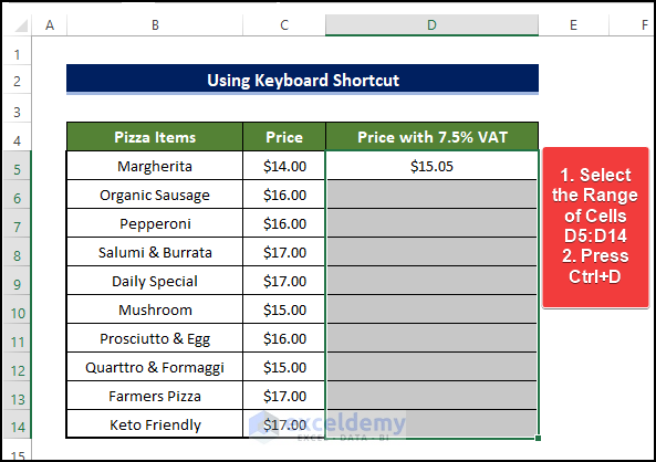
- This will fill the range of cells D5:D14 with the formula mentioned in cell D5.

Download the Practice Workbook
Related Articles
- [Fix] Excel Fill Series Not Working
- How to Auto Number or Renumber after Filter in Excel
- How to AutoFill Numbers in Excel with Filter
- How to AutoFill Ascending Numbers in Excel
<< Go Back to Autofill Numbers | Excel Autofill | Learn Excel
Get FREE Advanced Excel Exercises with Solutions!

Awesome!!!