Method 1 – AutoFill Ascending Numbers Using the Fill Handle in Excel
STEPS:
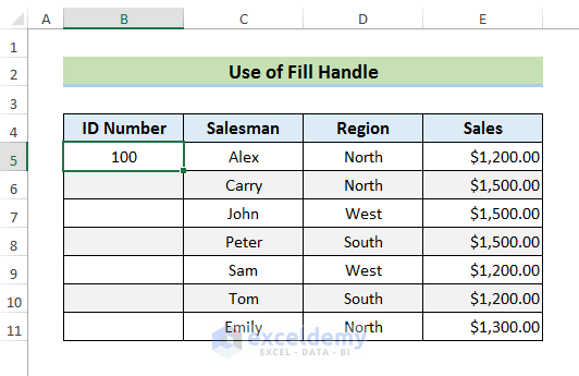
- Select a cell and enter the first number manually. Here, B5 and 100.
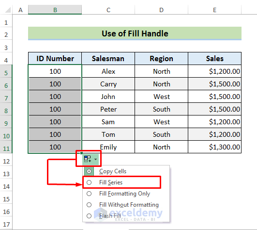
- Drag down the Fill Handle or double-click it. The ‘AutoFill Options’ will be displayed.
- Select Fill Series.
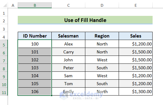
The rest of the cells will be filled in ascending order.
- To maintain a step value, enter the first two values and select them. Here, 100 and 105 in B5 and B6.
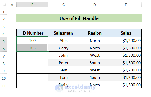
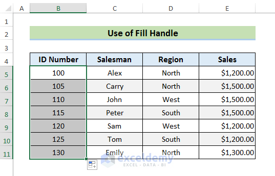
- Use the Fill Handle to see the result.
Read More: How to AutoFill Numbers in Excel
Method 2 – Using the Fill Command to AutoFill Ascending Numbers
STEPS:
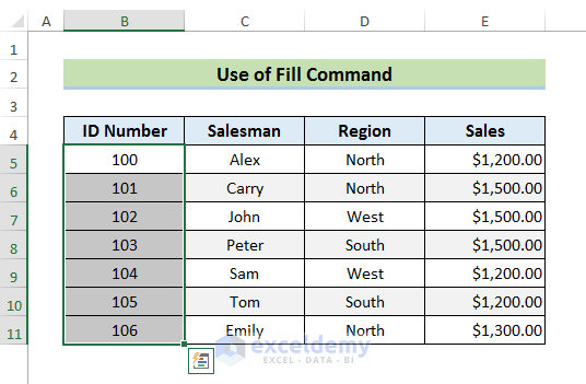
- Select a cell and enter the first number.
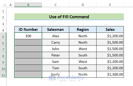
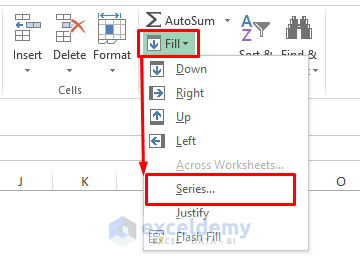
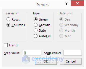
- Go to the Home tab and select Fill.
- Choose Series.
- Click OK.
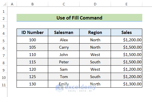
You will see an ascending series of numbers.
- To change the step value, use the ‘Series’ window.
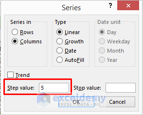
Here, the step value is 5. You can also select the stop value. If you need a geometric ascending pattern select ‘Growth’ in the Type field.
- Click OK to see the result.
Method 3 – Filling Ascending Numbers by Skipping a Row in Excel
STEPS:
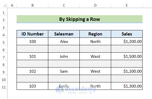
- Enter the first number manually in the first cell. Here, 100 in B5.
- Select B5 and B6.
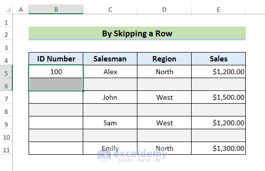
- Drag down the Fill Handle.
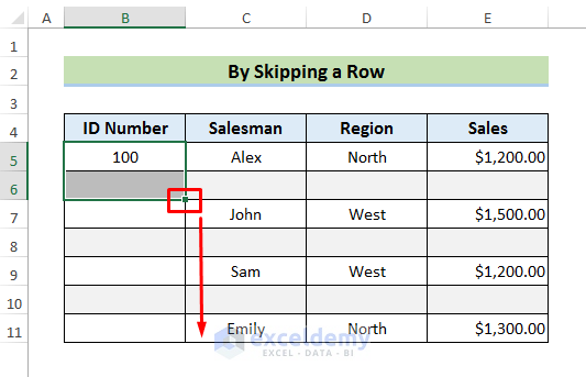
- You will see the result.
Method 4 – AutoFilling Ascending Numbers with Formulas
4.1 Using the ROW Function
STEPS:
- Select B5.
- Enter the formula:
=ROW()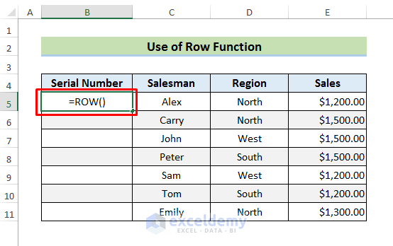
- Press Enter to see the result.
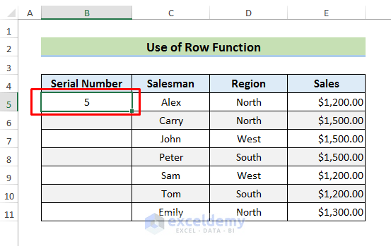
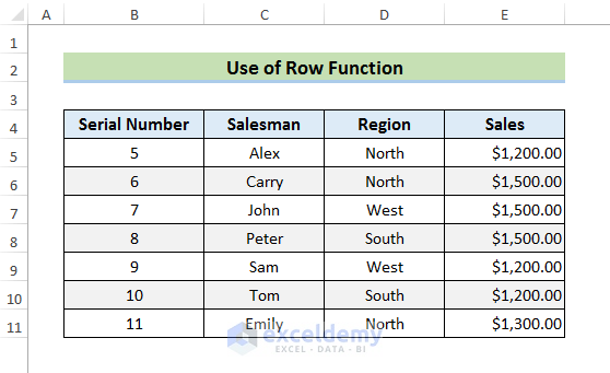
Here, the ROW Function displays the row number of the cell containing the formula.
- Use the Fill Handle to see the result.
- To start numbering from 1, enter:
=ROW(B1)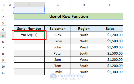
The ROW Function displays the row number B1.
- Press Enter to see the result.
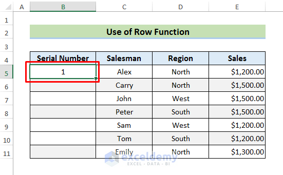
- Use the Fill Handle to see the final output.
Read More: How to AutoFill Numbers in Excel with Filter
4.2 Using the OFFSET Function
STEPS:
- Select B6.
- Enter the formula:
=OFFSET(B6,-1,O)+1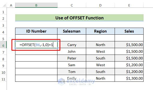
The OFFSET Function takes the value of the previous cell and adds 1 to it. The value of B5 is 0 because it is empty.
- Press Enter to see the result.
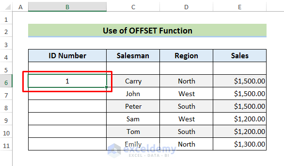
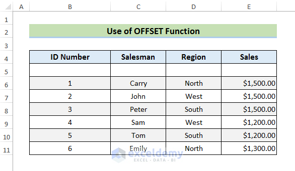
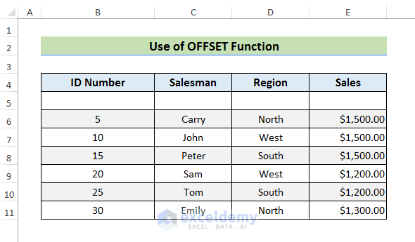
- Use the Fill Handle to see the ascending numbers.
- To start numbering from 5, add 5 instead of 1 in the previous formula.
=OFFSET(B6,-1,0)+5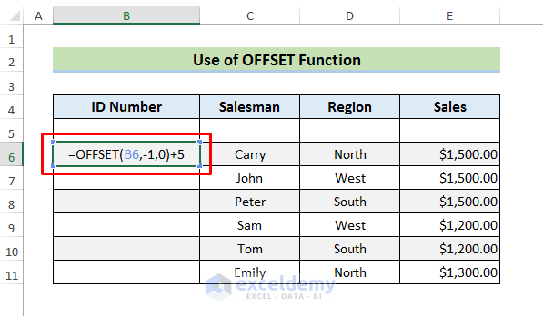
- Press Enter and drag down the Fill Handle to see the result.
Read More: How to Auto Number Cells in Excel
4.3 Using the COUNTA Function
STEPS:
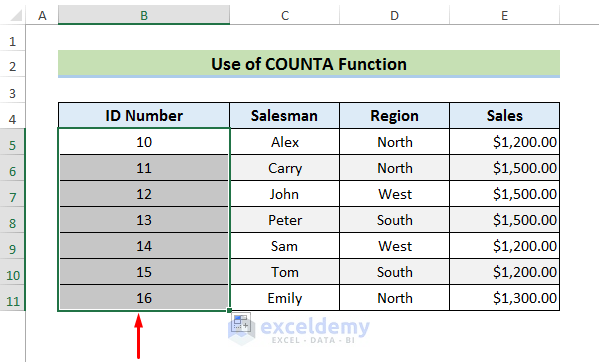
- Select B5 and enter the formula:
=COUNTA($C$5:C5)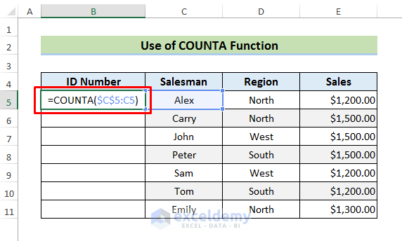
C5 was locked, using the dollar ($) sign. The COUNTA Function is applied to the given range.
- Press Enter and use the Fill Handle to see the result.
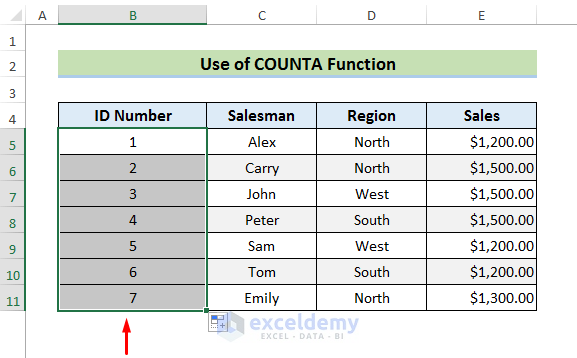
- To start numbering from 10, add 9 to the formula.
=COUNTA($C$5:C5)+9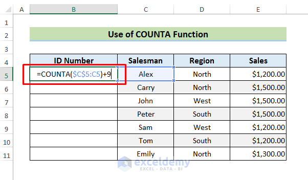
- Press Enter and use the Fill Handle to see the result.
4.4 Using the SUBTOTAL Function
STEPS:
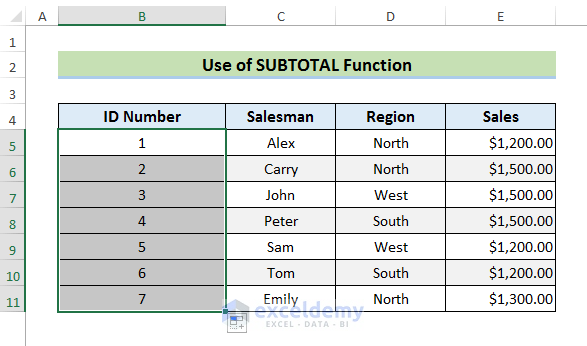
- Select B5 and enter the formula below.
=SUBTOTAL(3,$C$5:C5)
3 specifies the use of COUNTA and the second argument describes the range in which the SUBTOTAL Function is applied.
- Press Enter and then use the Fill Handle.
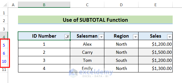
- If you use Filter and hide some rows, the ascending numbers will automatically be updated.
4.5 Adding 1 to the Previous Row
STEPS:
- Enter a value manually in the first cell. Here, 1 in B5.

- Enter the formula:
=B5+1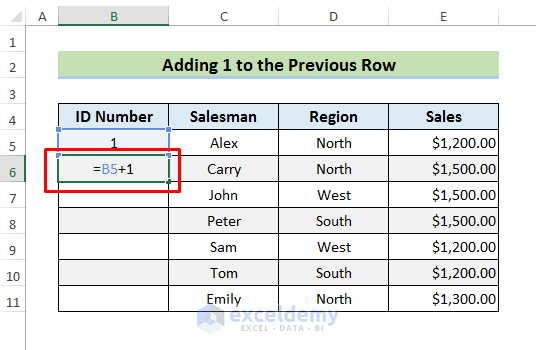
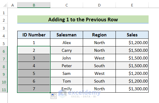
- Press Enter and use the Fill Handle to see the result.
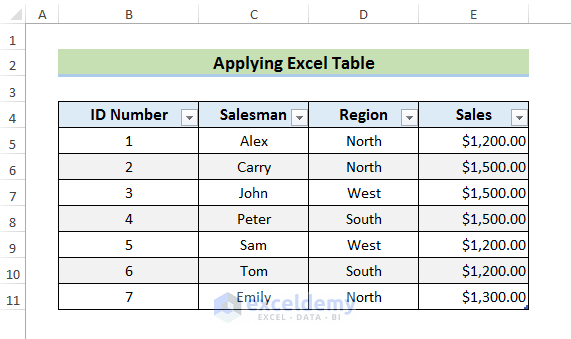
Method 5 – Applying an Excel Table to AutoFill Ascending Numbers
STEPS:
- Select any cell in your dataset.
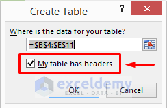
- Go to the Insert tab and select Table.

- In Create Table, select ‘My table has headers’.
- Click OK.
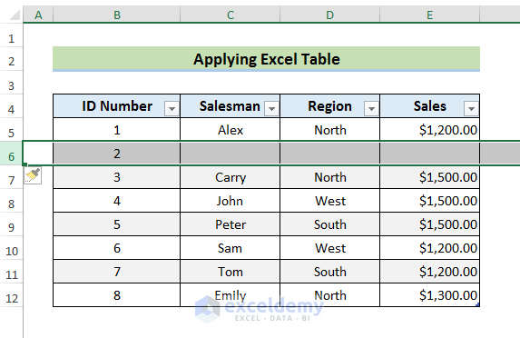
- Enter this formula in B5.
=ROW()-ROW(Table2[#Headers])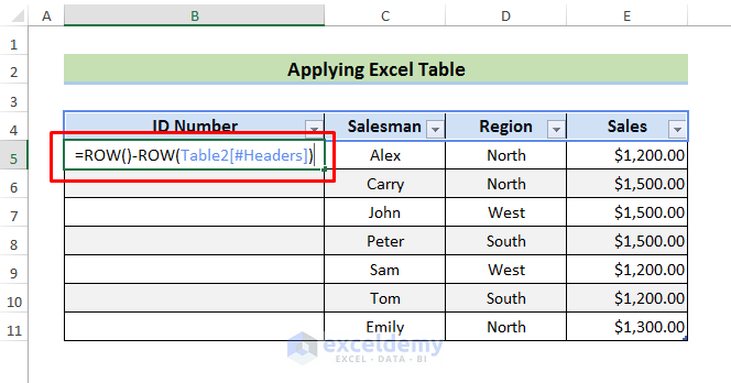
- Press Enter to see the result.
- If you insert a new row, the ascending numbers will automatically be updated.
Download Practice Book
Download the practice book here.
Related Articles
- How to Autofill Numbers in Excel Without Dragging
- Drag Number Increase Not Working in Excel
- How to Auto Number or Renumber after Filter in Excel
- [Fix] Excel Fill Series Not Working
<< Go Back to Autofill Numbers | Excel Autofill | Learn Excel
Get FREE Advanced Excel Exercises with Solutions!
