How to Use COUNTA Function with Criteria in Excel (4 Methods)

While working with a large dataset, sometimes we need to know the total number count of some certain dataset no matter whether it is a text or numbers or error or any other conditions. In Excel, you can do that with the COUNTA function. This article will show you how to use the COUNTA function with criteria in Excel with four methods.

The COUNTA Function in Excel

The COUNTA function in Excel counts all the non-empty cells including numbers, text, errors, empty text (“”), formula with null returning value, etc.

Generic Formula:

Where,

Below here we will learn different criteria to implement COUNTA Functions in Excel.

How to Utilize COUNTA Function with Criteria in Excel: 4 Ways

This section will further discuss four different applications, where you can implement COUNTA function with criteria in Excel to calculate non-equal cells to a range of certain things, to calculate the number of non-blank cells without zero (0) and with a formula returning a null value, how to achieve automatic summation after adding values in a table array and how to produce segmentation statistics by utilizing the COUNTA function.

Criteria 1. Using COUNTA Function to Count Non-Equal Cells to a Range of Certain Things in Excel

Suppose, you want to count cells that are not equal to a range of certain things.

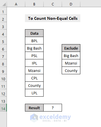
For instance, in the dataset above, we had the name of Cricket Premier leagues from where we wanted to count how many numbers of cells have similar kinds of names. So, we exclude Big Bash, Mzansi, and County in another table and apply the following formula,

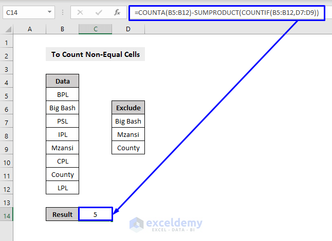
Which showed us the counted result of how many data are there in the original column.

Formula Breakdown:

 Let’s break the formula down to understand what happened inside the calculations,

• COUNTIF(B5:B12,D7:D9) -> holds values that we don’t want to count (D7:D9) and generates a count in a range of cells (B5:B12).

Output: 1, 1, 1

• SUMPRODUCT(COUNTIF(B5:B12,D7:D9)) -> sums up all the items that we got from the above COUNTIF formula.

Output: 3

• COUNTA(B5:B12)-SUMPRODUCT(COUNTIF(B5:B12,D7:D9)) -> based on the above output from the SUMRODUCT function, it actually refers COUNTA(B5:B12)-3, which means it subtracts the summation of the count value of the things that we don’t to count from the original total to get the final result.

Output: 5

So that means, without Big Bash, Mzansi, and County in the original dataset, the final data count is 5.

Read More: Dynamic Ranges with OFFSET and COUNTA Functions in Excel

Criteria 2. Utilizing COUNTA to Count Non-Blank Cells without Zero (0) and with a Formula Returning Null Value in Excel

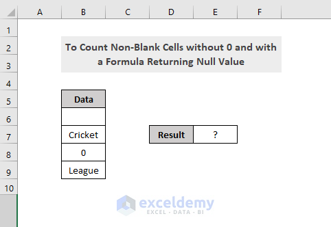
Suppose you have a dataset with a lot of important information, but that dataset also has some unnecessary values such as zero (0) and a formula that returns a null value. So, you want to know how much important information your dataset is holding without all those irrelevant values.

For instance, In the given dataset below, we wanted to know how many non-blank cells were there without any zero and formula returning a null value. 

In the cell B6, we have a formula that is returning null value (see the picture below)

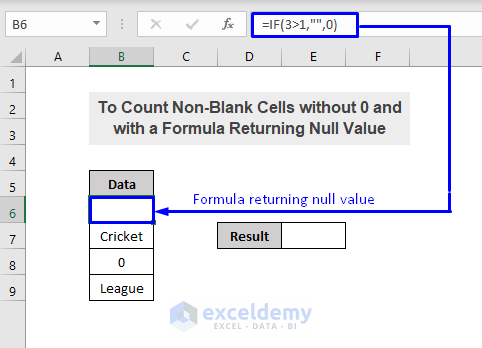
And we implemented the following formula to extract the result.

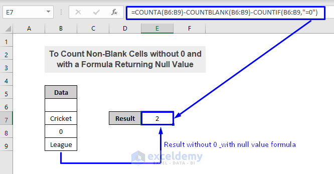
that showed us that we have 2 data in the data table that are without any zero and null value returning formula.

Formula Breakdown:

Let’s break the formula down to understand what happened inside the calculations,

• COUNTIF(B6:B9,”=0″) -> counts how many zeros are there in the selected data range (B6:B9).

Output: 1

• COUNTBLANK(B6:B9) -> Counts how many blank data are in the selected data range (B6:B9).

Output: 1

• COUNTA(B6:B9) -> Counts how many non-empty data are actually in there.

Output: 4

• So the final formula, COUNTA(B6:B9)-COUNTBLANK(B6:B9)-COUNTIF(B6:B9,”=0″) -> actually indicates 4-1-1

Output: 2

So we have 2 data in our dataset that are without any zero and null value returning formula.

Criteria 3. Applying COUNTA Function to Achieve Automatic Summation after Adding values in Excel

What if you have a huge dataset of sales value and the summation of those large datasets. If you want to add a new sale value, you have to update the whole dataset to add that newly added value.

But with the help of the COUNTA function, you can keep continuing to add new sales values and the total value will automatically keep updating. But to achieve that, the COUNTA function needs a little help from other Excel functions as well.

The formula:

The above formula is based on the below dataset that shows the detailed calculation of how to achieve automatic summation after each added value.

Formula Breakdown:

• COUNTA(C:C) -> used to count the total number of cells in the whole column C.

Output: 6, which is exactly the total number of cells in C4:C9.

• COUNTA(C:C)-1) -> subtracts 1 to remove the header cell.

Output: 5

• OFFSET(C4,1,,COUNTA(C:C)-1) -> actually becomes OFFSET(C4,1,,5) which returns to the reference to cells 1 row under C4 and 0 column to the right of C4 and height to 5 that is the reference to C5:C9

• SUM(OFFSET(C4,1,,COUNTA(C:C)-1)) -> becomes SUM(C5:C9) and add each number in C5:C9 to get the final result.

When adding a new value in the bottom cells, notice that the result value in cell F7 is automatically updating.

What is happening here is, when a new number is added in cell C10, the last row of column C, the counted result of COUNTA(C:C) becomes 7, 7 minus 1 becomes 6, then offset returns C4:C9, so every time a row is added after the table, the formula will automatically add it.

Read More: [Fixed] Excel COUNTA Function Not Working

Criteria 4. Producing Segmentation Statistics by Utilizing COUNTA Function in Excel

If you want to count the number of sales in January and February month of your company, using the COUNTA formula is a great way to do it combining with some other functions.

The formula to do that is,

 And the dataset,

Formula Breakdown:

• (ROW()-5)/4)*4 -> here 4 means that one segment in the table array is four rows, ROW() returns the row number 5 of the cell where the formula is located and then returns 0.

• INT((ROW()-5)/4)*4 -> Int function is used for rounding which returns 0.

• OFFSET($D$5:$D$8,INT((ROW()-5)/4)*4, ) -> actually becomes OFFSET(($D$5:$D$8, 0*4), which returns the reference to cells 0 row under D5 and 0 column to the right of D5 and the same height and width as D5:D8, returning as table array.

• COUNTA(OFFSET($D$5:$D$8,INT((ROW()-5)/4)*4, )) -> becomes COUNTA(($D$5:$D$8).

Output: 4

• IF(MOD(ROW()-5,4)=0, COUNTA(OFFSET($D$5:$D$8,INT((ROW()-5)/4)*4, )),””) -> becomes IF(MOD(ROW()-5,4)=0, 4, “”), since ROW() returns 5, MOD(ROW()-5,4) becomes MOD(5-5, 4), then use the Mod function to modulo 0 and 4, the result is 0; then the formula becomes =IF(0=0,4,””), since the condition 0=0 of if function is established, it returns 4.

Once you are done with the first segment (January month) of your data table, simply drag the row down using Fill Handle to apply the following formula in the result of the cells and to count how many sales you had in each month.

Download Practice Template

You can download the free practice Excel template from here and practice on your own.

Conclusion

This article explained in detail how to implement the COUNTA functions with criteria in Excel to solve various problems that we encounter in our life. I hope this article has been very beneficial to you. Feel free to ask any questions if you have regarding the topic.

Related Articles

• How to Use COUNTA from SUBTOTAL Function in Excel
• Difference Between COUNT and COUNTA Functions in Excel

<< Go Back to Excel COUNTA Function | Excel Functions | Learn Excel