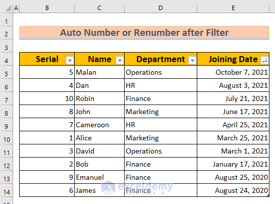
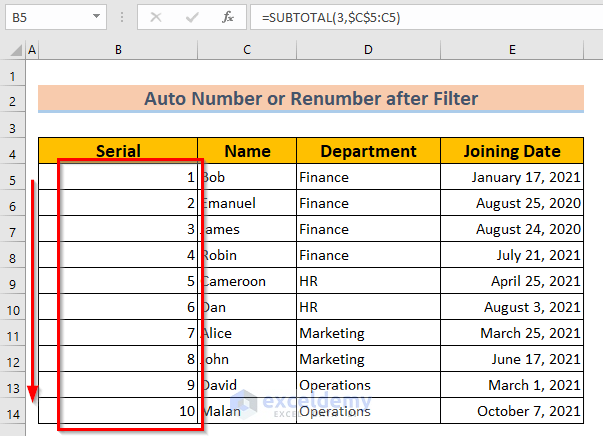
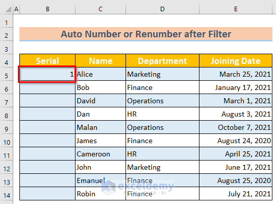
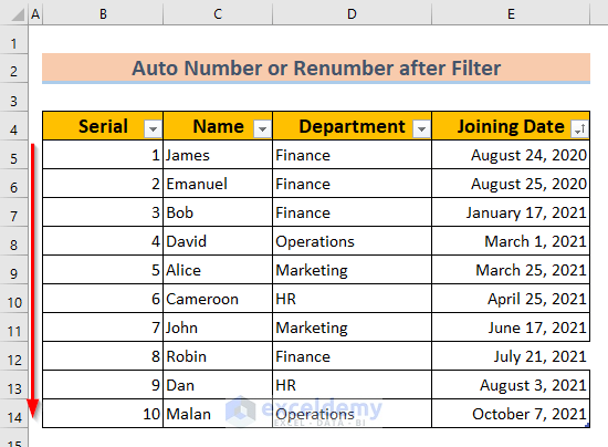
Suppose a company has employee records in a worksheet. The worksheet has four columns: Serial, Name, Department, and Joining Date. The company might need to arrange the data according to departments or joining dates. If we Filter according to Joining Date, the serial numbers get jumbled. Let’s see how we can make the serial numbers get auto-renumbered after filtering.
How to Auto-Number or Renumber after Filter in Excel: 7 Easy Ways
Method 1 – Using SUBTOTAL to Auto-Number or Renumber after a Filter in Excel
Steps:
- In cell B5, copy the following formula:
=SUBTOTAL(3,$C$5:C5)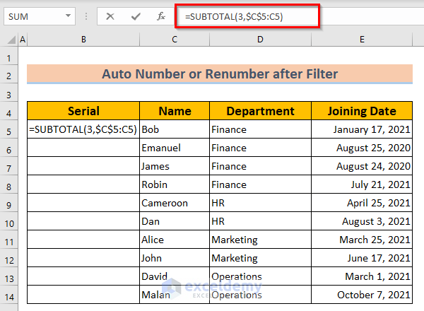
Formula Breakdown
$C$5:C5>> This denotes an expanding range. The first element of the range is locked, so the first element will always remain the same. The second element will change if we drag down the formula.
Output is>> C5:C5
Explanation>> Here, only one cell contains in the range.
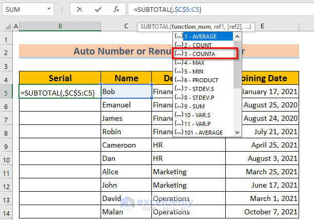
3,$C$5:C5>> In this case, 3 denotes the COUNTA function. In the picture below we have given a list of numbers that denote different functions in the case of the SUBTOTAL function.
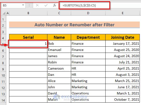
SUBTOTAL(3,$C$5:C5)>> Gives us the total of cells with values in the selected range.
Output is>> 1
Explanation>> There is only one cell with a value in the C5:C5 range.
- Press Enter to get the first result.
- Drag down or double-click the Fill Handle to AutoFill to the rest of the column.
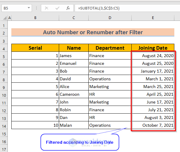
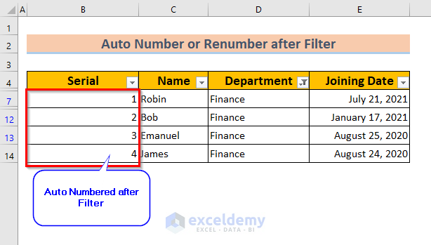
- If we arrange the cells according to Joining Date using a Filter, we will see that the serial numbers get sorted automatically.
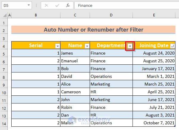
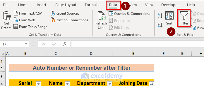
- To Filter, click on the arrow in the header of the table.
- Go to the Data tab and click Filter.
- Select Finance.
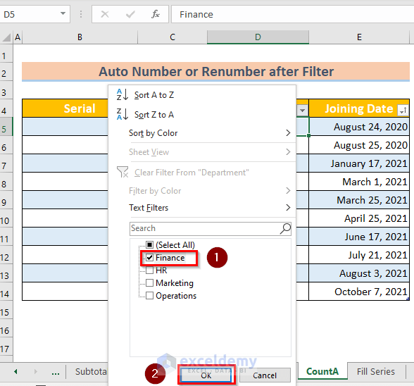
- If we filter data and choose the Finance department, the resultant rows will be numbered automatically.
Read More: How to AutoFill Numbers in Excel with Filter
Method 2 – Auto-Number or Renumber after Filtering with a Combined Formula
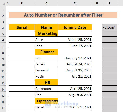
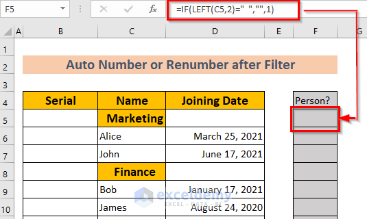
In this method, the dataset has been further sorted by department. Each department name has two spaces before the text, which we’ll use to determine if the row corresponds to a person or is used for sorting. We’ll use the helper column to create auto-incrementing serial numbers.
Steps:
- Copy the following formula to the cell F5:
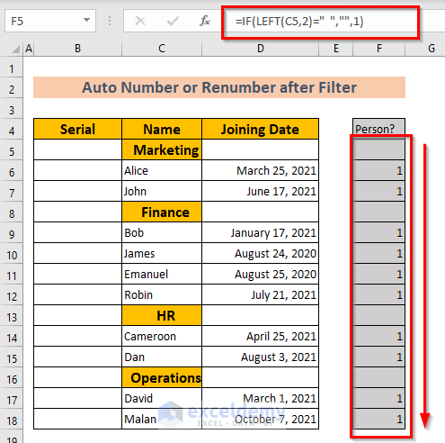
=IF(LEFT(C5,2)=" ","",1)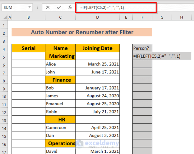
Formula Breakdown
LEFT(C5,2)>> Fetches two characters from the left of cell C5.
Output is>> Double space
LEFT(C5,2)=" ">> This logical test denotes whether the left two characters of cell C5 are two spaces or not.
Output is>> TRUE
Explanation>> The left two characters are equal to double spaces.
IF(LEFT(C5,2)=" ","",1)>> The IF function returns a value blank if the above condition is satisfied. Otherwise, it returns the value 1.
Output is>> Blank
Expanation>> In this case the left two characters are double space.
- Hit Enter.
- Drag down the Fill Handle to AutoFill. Double-clicking might not work since the formula doesn’t always provide an output.
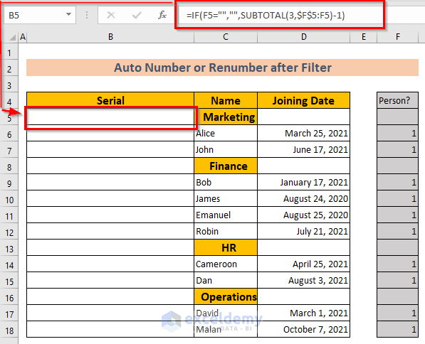
- Insert the following in the B5 cell:
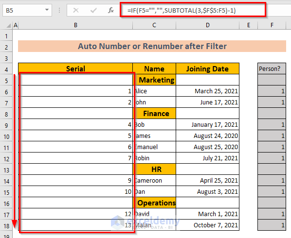
=IF(F5="","",SUBTOTAL(3,$F$5:F5)-1)
Formula Breakdown
F5="">> Determines whether the value in F6 cell is blank.
Output is>> TRUE
Explanation>> F5 cell is blank.
SUBTOTAL(3,$F$5:F5)-1>> Returns value of the expandable range $F$5:F5 as shown in method 1.
IF(F5="","",SUBTOTAL(3,$F$5:F5)-1)>> The IF function returns the value blank if the above condition is satisfied. It gives the value of SUBTOTAL(3,$F$5:F5)-1 if the corresponding cell is in Person? The column is not blank.
Output is>> Blank
Explanation>> F5 cell is blank.
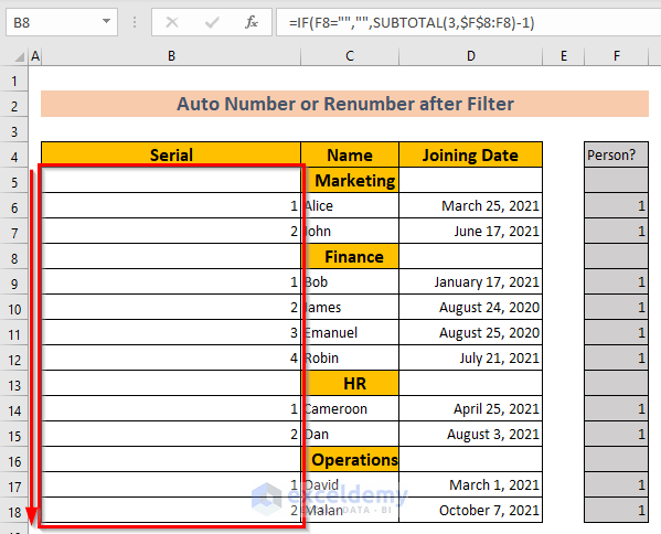
- Press Enter.
- Drag down or double-click the Fill Handle to AutoFill column B.
- If you want the serial number to start from 1 for every department, you need to adjust the formula. For Finance in the example, the starting range will be:
$F$8:F8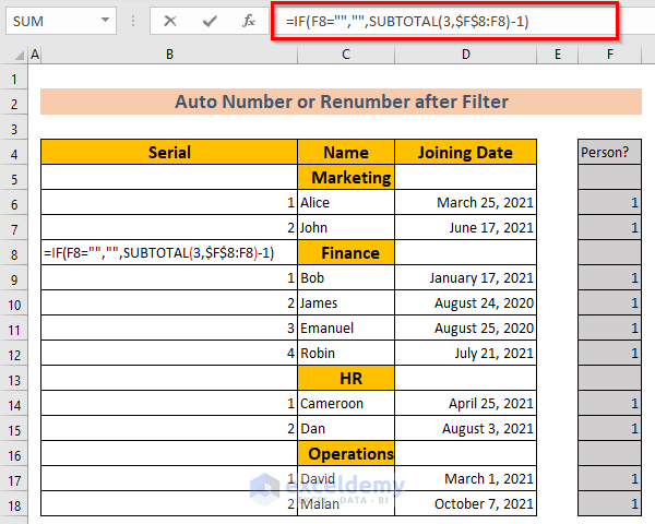
- You’ll need to manually change the formula for all departments and drag down the Fill Handle.
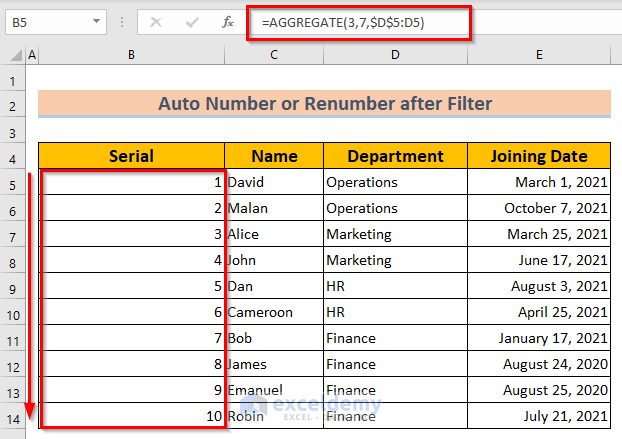
Method 3 – Auto-Number or Renumber after Filtering Using the AGGREGATE Function
Steps:
- In cell B5, copy the following formula:
=AGGREGATE(3,7,$D$5:D5)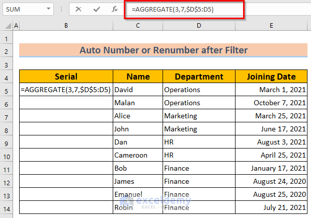
Formula Breakdown
$D$5:D5>> Denotes the expandable range
3>> Denotes COUNTA function
7>> Denotes Ignore Hidden Rows and Error Values
AGGREGATE(3,7,$D$5:D5)>> Denotes the sum of COUNTA excluding hidden rows and error values
- Hit Enter.
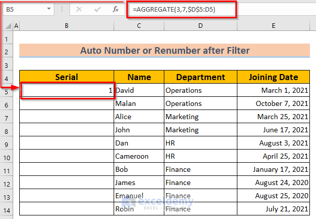
- Drag down or double-click the Fill Handle to AutoFill the column.
- Use a Filter to filter out some of the data, and the serial numbers will change automatically.
Read More: [Fix] Excel Fill Series Not Working
Method 4 – Using the ROW Function to Auto-Number or Renumber after Filtering
STEPS:
- Insert the following formula in B5:
=ROW()-4 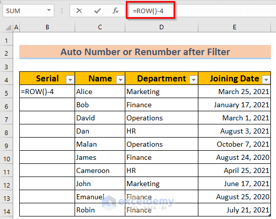
Formula Breakdown
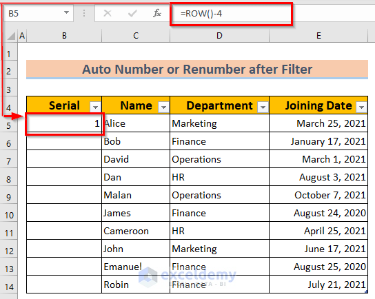
ROW()>> Denotes the number of rows.
Output is>> 5
Explanation>> B5 cell is in row 5
ROW()-4>> Denotes the number after subtracting 4
Output is>> 1
Explanation>> 5-4
- Hit Enter.
- AutoFill the column via the Fill Handle.
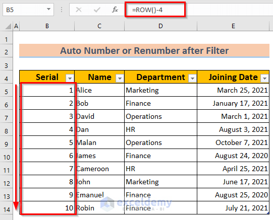
- Once you use a filter, the formula recalculates the serial numbers accordingly.
Method 5 – Auto-Number or Renumber after Filtering with the COUNTIF Function
STEPS:
- Insert the following formula in cell B5:
=COUNTIF($D$5:D5,D5)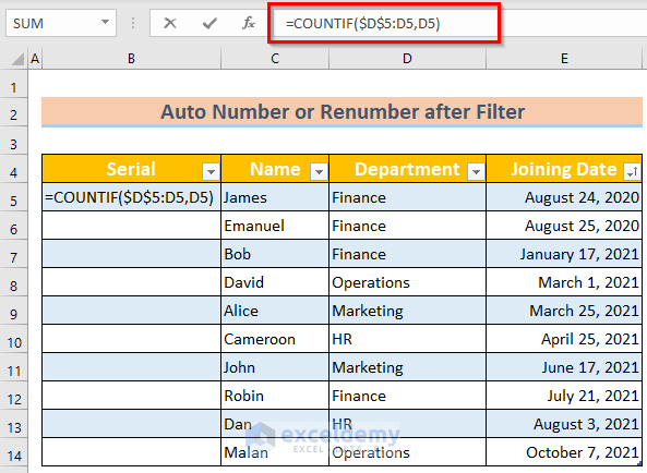
Formula Breakdown
$D$5:D5>> Denotes the expandable range
D5>> Denotes the value in D5 cell
Output is>> Finance
COUNTIF($D$5:D5,D5)>> The COUNTIF function counts the number of cells with the value of D5 cell
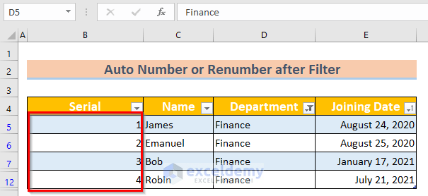
- Press Enter.
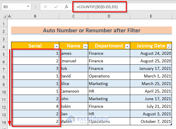
- If we choose any department by filtering the Department column, we will get the correct serial numbers.
Read More: How to Autofill Numbers in Excel Without Dragging
Method 6 – Using Fill Series to Auto-Number or Renumber after a Filter
Steps:
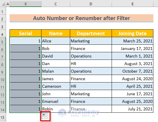
- Make the Serial column blank.
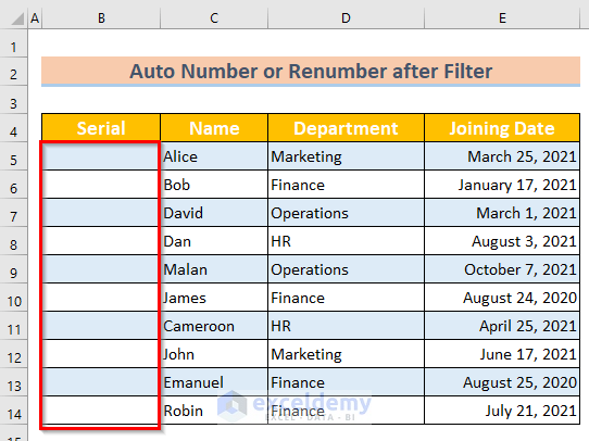
- Select the entire Serial column.
- Put 1 in the first cell.
- Fill all the cells of the column using Fill Handle.
- Go to the AutoFill Options as shown in the picture below. If your autofill option menu is not showing you can turn it on from the Options menu.
- Select Fill Series.
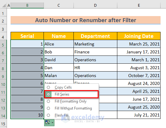
- The correct order of serial will appear.

- Filter your data, and the column will auto-recalculate.
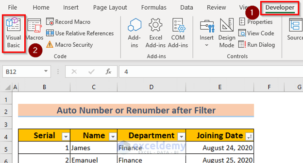
Method 7 – Auto-Number or Renumber after a Filter Using VBA
Steps:
- Open the Developer tab and select Visual Basic
- A new window will open.

- Go to Insert and select Module.
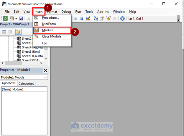
- A new Module will open.

- Copy the code below and paste it into the Module.
Sub Autonumbering()
Dim X As Range
Dim Y As Range
On Error Resume Next
xTitleId = "Autonumbering"
Set Y = Application.Selection
Set Y = Application.InputBox("Range", xTitleId, Y.Address, Type:=8)
Set Y = Y.Columns(1).SpecialCells(xlCellTypeVisible)
xIndex = 1
For Each X In Y
X.Value = xIndex
xIndex = xIndex + 1
Next
End Sub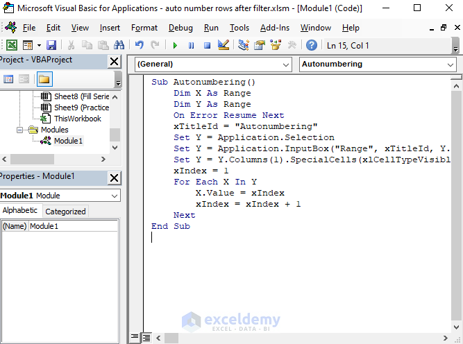
Here, we have initiated a Sub Procedure named Autonumbering. We have declared two variables X and Y. Both variables are Range type. We have used For Loop to go to the next cell.
Also use On Error Resume Next to continue while occurring any error.
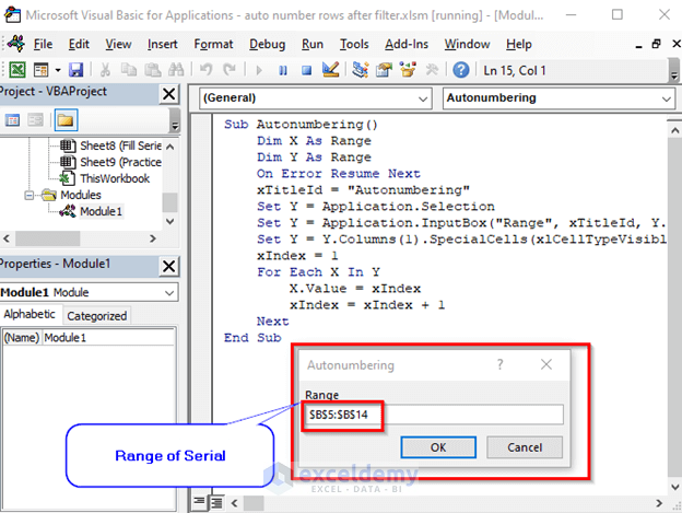
- Select Run Sub/UserForm or use the F5 key to run the code.
- A new dialogue box will appear. Type the range over which you want to put a correct serial number.
- You will get the correct serial in the Serial column.
- Apply a filter and check if the column is automatically renumbered.
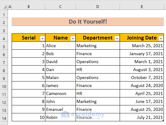
Practice Section
We have included a practice section in the worksheet provided which you can use to implement these methods.
Download the Practice Workbook
Related Articles
- Drag Number Increase Not Working in Excel
- How to AutoFill Ascending Numbers in Excel
- How to Auto Number Cells in Excel
<< Go Back to Autofill Numbers | Excel Autofill | Learn Excel
Get FREE Advanced Excel Exercises with Solutions!
