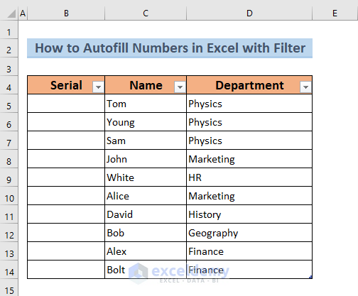
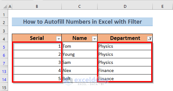
We have the Names of some students along with their Department. In the Serial column, we are going to list the students serially with Filter activated.
Method 1 – AutoFill Numbers in Excel with a Filter Using the SUBTOTAL Function
STEPS:
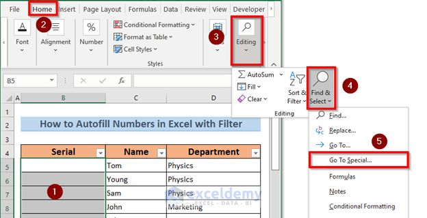
- Select the cell range B5:B14.
- Open the Home tab and go to Editing.
- From Find & Select, choose Go To Special.
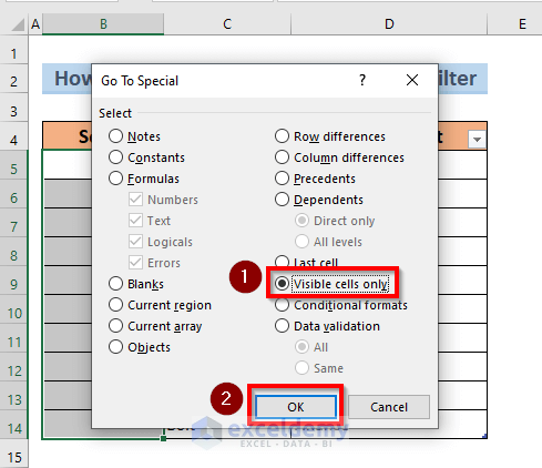
- A dialog box will pop up.
- Select Visible cells only and click OK.
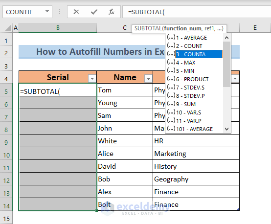
- Use this formula in the first selected cell or in the Formula bar.
=SUBTOTAL(3,$C$5:C5)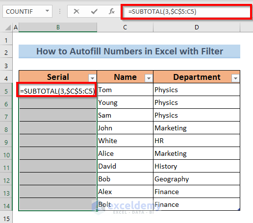
Formula Breakdown
$C$5:C5 >> This denotes an expanding range. The first element of the range is locked, so the first element will always remain the same. The second element will change if we drag down the formula.
Output is>> “Tom”
Explanation>> Here, it is the cell value of the C5 cell.
3,$C$5:C5 >> In this case, 3 denotes the COUNTA function. In the picture below we have given a list of numbers that denote different functions in the case of the SUBTOTAL function.
SUBTOTAL(3,$C$5:C5) >> Gives the total of cells with values in the selected range.
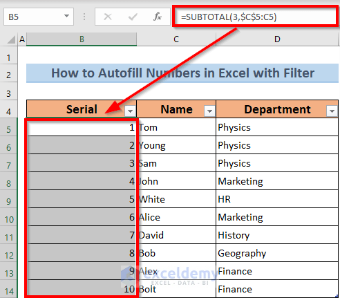
Output is >> 1 2 3 4 5 6 7 8 9 10
Explanation>> Returns a range of numbers for the selected cell range
- Press Ctrl + Enter as it’s an array formula.
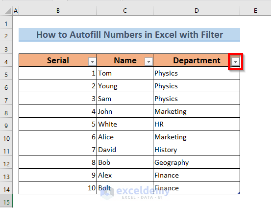
- Filter the dataset with Physics and Finance in the Department. Click the filter icon.
- Select Physics and Finance.
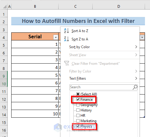
- Excel will recalculate the Serials sequentially.
Read More: How to Auto Number or Renumber after Filter in Excel
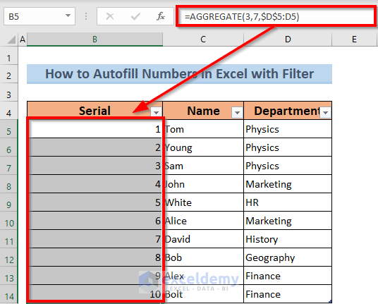
Method 2 – Using the AGGREGATE function to AutoFill Numbers with a Filter
STEPS
- Apply Visible cell only to the range you are going to work with by following Method 1.
- Use the following formula in the Formula bar
=AGGREGATE(3,7,$D$5:D5) 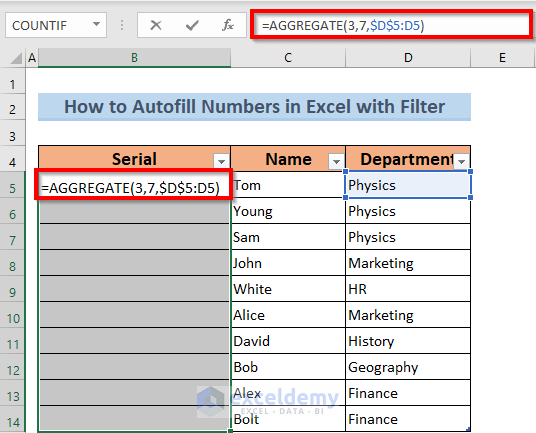
Formula Breakdown
$C$5:C5 >> This denotes an expanding range. The first element of the range is locked, so the first element will always remain the same. The second element will change if we drag down the formula.
Output is >> “Tom”
Explanation >> Here, it is the cell value of C5 cell.
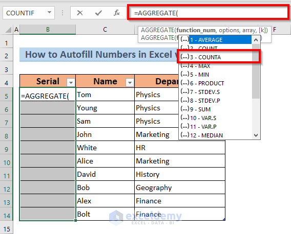
3,7,$C$5:C5 >> In this case, 3 denotes the COUNTA function. We have shown the list of functions that Excel shows in the image below.
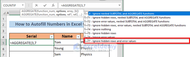
In this case, 7 denotes the option Ignore hidden rows and error values. In the picture below, we have given a list of numbers that denote different options for the AGGREGATE function.
AGGREGATE(3,7,$C$5:C5) >> Returns the Serial numbers for the selected range.
Output is >> 1 2 3 4 5 6 7 8 9 10
Explanation >> Returns a range of numbers for the selected cell range.
- Press Ctrl + Enter as it’s an array formula.
- Filter from the Department column by selecting Physics and Finance like in Method 1.
- Excel will rearrange the Serial numbers.

Read More: How to Auto Number Cells in Excel
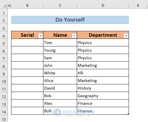
Practice Workbook
We have attached a practice sheet for you to practice.
Download the Practice Workbook
Related Articles
- How to Autofill Numbers in Excel Without Dragging
- Drag Number Increase Not Working in Excel
- How to AutoFill Ascending Numbers in Excel
- [Fix] Excel Fill Series Not Working
<< Go Back to Autofill Numbers | Excel Autofill | Learn Excel
Get FREE Advanced Excel Exercises with Solutions!

I have a list of library books with various headings subheadings and comments interspersed with the data.
I can filter these out by selecting a column that only contains data if the line is an entry for a library book.
So I want to apply the filter (which I can do using your methods) but I want that number to be permanent regardless of what filter i apply.
Hi David
As far as I understand the case, you want to apply a filter to a row but keep the numbers in the cell permanent.
Unfortunately, when Excel executes a filter, it hides the entire row. If any cell contains numbers, excel will hide them too. However, as this article explains, you can maintain the serial when applying a filter.
In case I have misunderstood your requirement, please mail us the excel file at [email protected] and explain the problem a bit more.
Thank you.