Method 1: AutoFill a Column with a Series of Numbers
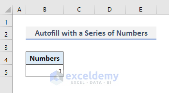
Example Model:
Use the Fill Handle option to autofill the series of numbers starting from 1.
Steps:
- Select Cell B5.
- Select the cell and find the Plus (+)
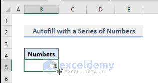
- Drag the Plus (+) icon downward.
- Click on the options menu and select the Fill Series
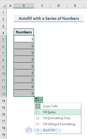
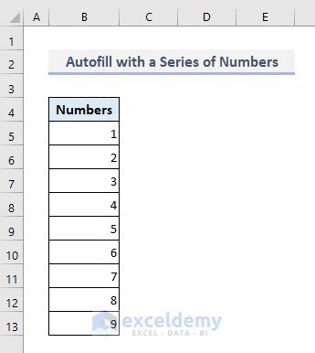
Note: A series of numbers will appear starting from 1 to 9.
Read More: How to Auto Number Cells in Excel
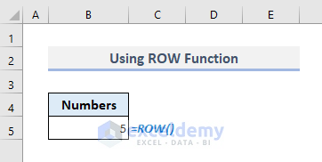
Method 2: AutoFill Numbers by Using the ROW Function in Excel
In the following picture, Cell B5 is situated in Row 5. So if you apply the ROW function in that cell, the function will return ‘5’.
Steps:
- Enter the following formula into cell
=ROW()-4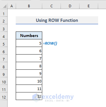
- To start the number with ‘1’, input the following formula in Cell B5:
=ROW()-4Note: Since the data was in the 5th row, the ROW function returned the number ‘5’. To replace it with number ‘1’, we have to subtract ‘4’ from the ROW function.
Method 3. Insert the OFFSET Function to AutoFill Numbers in a Column
Steps:
- Enter the following formula into cell
=OFFSET(B4,-1,0)+1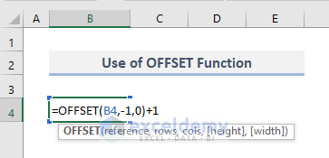
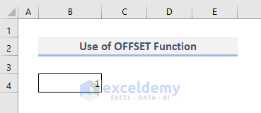
- After pressing Enter, the number ‘1’ will appear.
Note: Keep in mind that while using this formula immediate upper cell blank must be blank.
- Use the Fill Handle to autofill the column.
Note: You don’t have to choose the Fill Series option anymore as shown in the first method.

Read More: How to Autofill Numbers in Excel Without Dragging
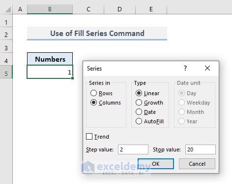
Method 4: AutoFill Numbers by Using the Fill Series Command
Steps:
- From the Home , go to the Editing group of commands.
- Select the Series command from the Fill drop-down under the Editing group of commands.
Note: A dialogue box named ‘Series’ will open up.

Let’s assume we want to create a series of numbers with a common difference of ‘2’ and the series will end with the last value of not more than 20.
- Select the Columns radio button from the Series in options.
- Input ‘2’ and ‘20’ in the Step value and the Stop Value.
- Press OK.
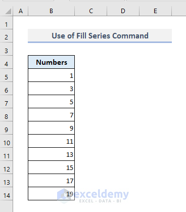
Note: You’ll find the series of numbers with the mentioned criteria right away.
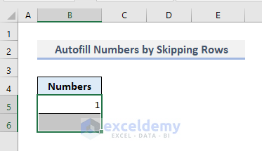
Method 5. AutoFill Numbers While Skipping Rows (Blank Cells)
Example Model:
Select two successive cells starting from the first input data as shown in the following screenshot.
Steps:
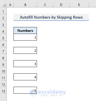
- After auto-filling the column with the Fill Handle, you’ll find the series of numbers starting with ‘1’ while skipping a row at regular intervals.
Method 6: AutoFill Formulas in a Column in Excel
Steps:
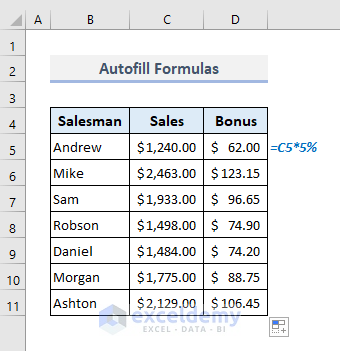
- Enter the following formula into cell D5.
=C5*5%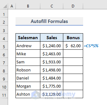
- Use the Fill Handle from Cell D5 and drag it down to Cell D11.
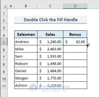
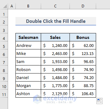
Method 7: Double-Click the Fill Handle to AutoFill Numbers
Steps:
- Click the Fill Handle icon in the right-bottom corner of Cell D5 twice.
Read More: How to AutoFill Numbers in Excel with Filter
Method 8: AutoFill Numbers using a Geometric Pattern
Steps:
- Open the Series dialogue box from the Fill options in the Editing group of commands.
- Select the Columns button as the Series in option.
- Choose Growth as the Type of the series.
- Input ‘2’ and ‘200’ as the Step value and the Stop value
- Press OK.
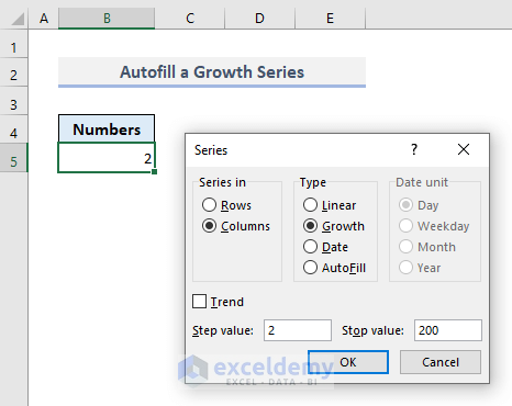
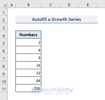
Note: You’ll find the geometric series starting from 2 with a growth rate of 2, which means each value will be multiplied by 2 until the final output exceeds 200.
Method 9: AutoFill a Date Series in a Column
- Select the Columns radio button from the Series in options.
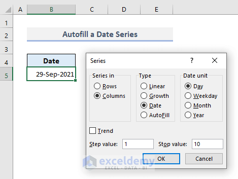
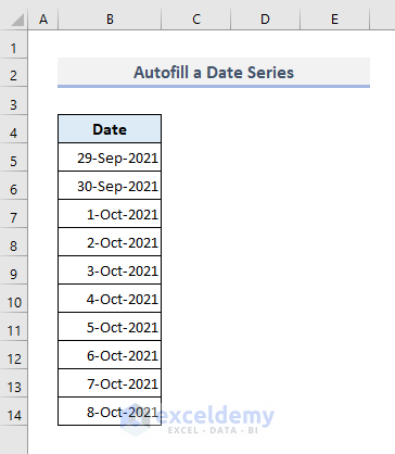
Note: After pressing OK the dates are as shown in the following picture.
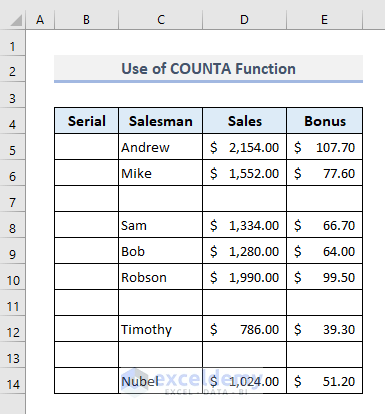
Method 10: AutoFill Row Numbers with COUNTA Function to Ignore Blank Cells
In the following picture, Column B will represent the serial numbers. We have to assign a formula in Cell B5, drag it down to the bottom, and define the serial numbers for all non-blank rows.
Steps:
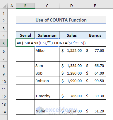
- Enter the following formula into cell B5.
=IF(ISBLANK(C5),””,COUNTA($C$5:C5))- Press Enter for the first serial number ‘1’ as the first row in the table is not empty.
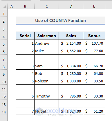
- Use the Fill Handle to autofill the entire Column B.
Note: The serial numbers for all non-empty rows appear at once.
Read More: Excel Formulas to Fill Down Sequence Numbers Skip Hidden Rows
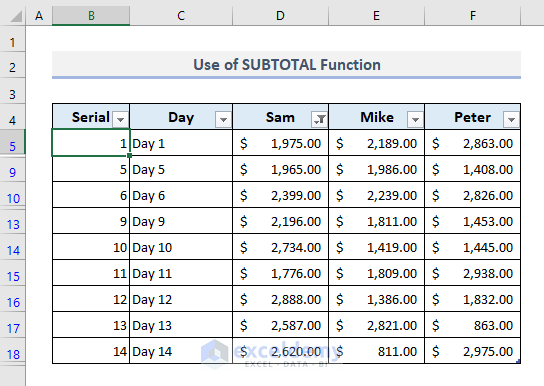
Method 11: Use the SUBTOTAL Function to AutoFill Numbers for Filtered Data
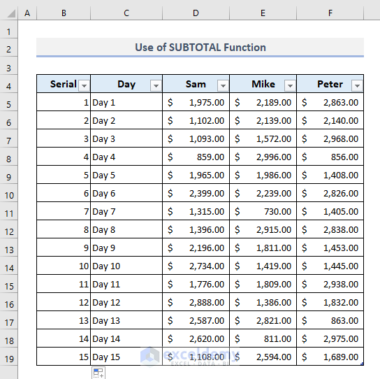
In the following table, we’ve filtered the data for Sam only. We’ve extracted the sales values of greater than $1500 for Sam here. However, after filtering the table, the serial numbers have also been modified. Let’s assume, we want to maintain the serial numbers as they were shown initially.
Steps:
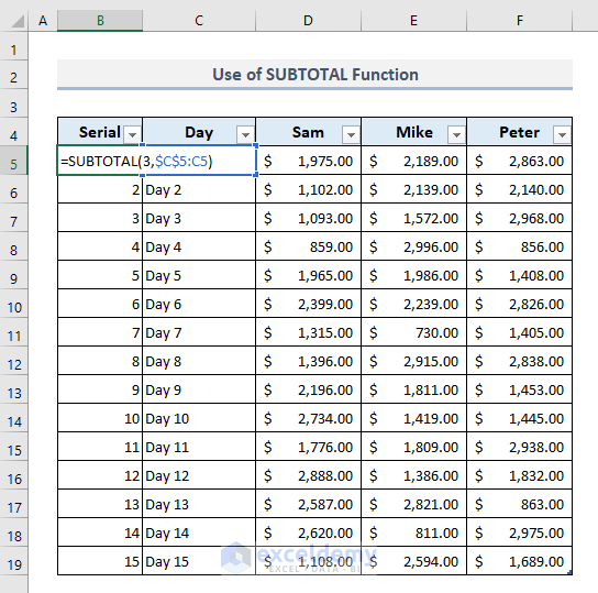
- Enter the following formula into cell B5.
=SUBTOTAL(3,$C$5:C5)- Use Fill Handle to autofill the entire column.
- Now filter the sales values of Sam to show the amounts that are greater than $1500 only.
Note: The serial numbers have not been modified here as they’re maintaining the sequence of the numbers.

Read More: How to Repeat Number Pattern in Excel
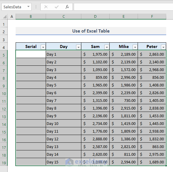
Method 12: Create an Excel Table to AutoFill Row Numbers (ROW Function)
Steps:
- Select the entire table data (B5:F19) and name it with Sales Data by editing in the Name Box.
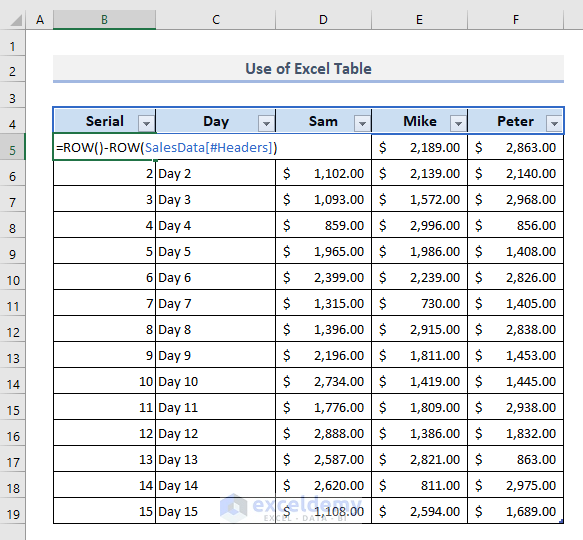
- Enter the following formula into cell
=ROW()-ROW(SalesData[#Headers])Note: The entire Column B in the data table will display the serial numbers.
- Right-click any of the row numbers on the left of the spreadsheet with your mouse cursor.
- Select the Insert option.
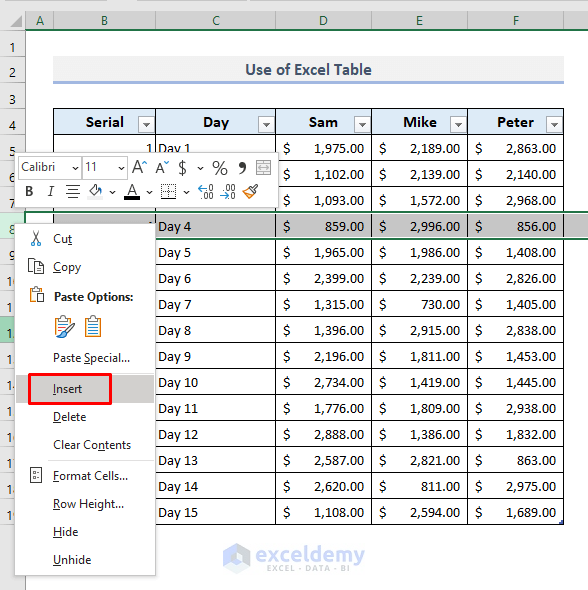
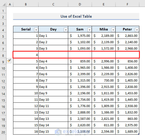
Note: A new row will be added in the selected region and the serial numbers of the entire data table will be updated simultaneously.
Download Practice Workbook
You can download the Excel workbook that we’ve used to prepare this article.
AutoFill Numbers in Excel: Knowledge Hub
- How to Add Sequence Number by Group in Excel
- How to AutoFill Ascending Numbers in Excel
- How to Auto Number or Renumber after Filter in Excel
<< Go Back to Excel AutoFill | Learn Excel
Get FREE Advanced Excel Exercises with Solutions!
