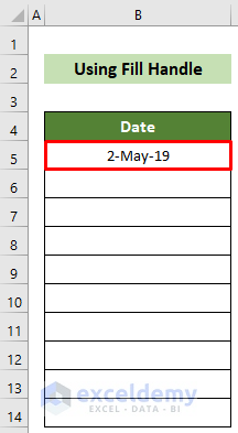
Consider the date: 2-May-19.
To automate the dates with rolling months:
Method 1 – Create Automatic Rolling Months Using the Fill Handle
Steps:
- Click B5 and enter the starting date.
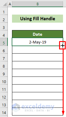
- Place the cursor at the bottom right corner of the cell.
- Drag down the Fill Handle.
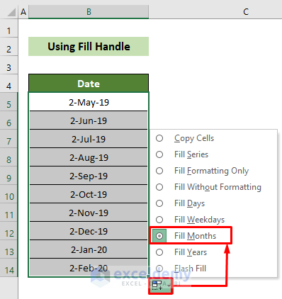
Cells will be filled with rolling dates. To display rolling months:
- Click the Fill Handle icon and choose Fill Months.
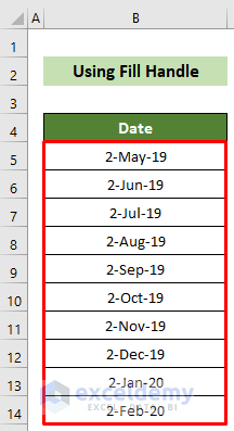
This is the output.
Read More: How to Repeat Formula Pattern in Excel
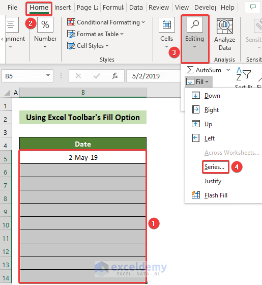
Method 2 – Using the Fill Option in the Excel Toolbar to Create Automatic Rolling Months
Steps:
- Click B5 and enter the starting date.
- Select B5:B14.
- Go to the Home tab >> Editing >> Fill >> Series…
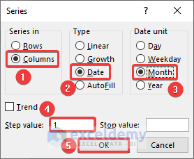
- Choose Columns in Series.
- Select Date in Type.
- Choose Month in Date unit.
- Enter 1 in Step value:.
- Click OK.
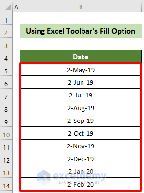
This is the output.
Read More: How to AutoFill Months in Excel
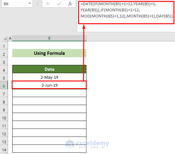
Method 3 – Using an Excel Formula with the DAY, DATE, MONTH, YEAR, IF, and MOD Functions
Steps:
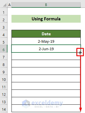
- Enter the starting in B5.
- Click B6 and enter the following formula.
=DATE(IF(MONTH(B5)+1>12,YEAR(B5)+1,YEAR(B5)),IF(MONTH(B5)+1>12,MOD(MONTH(B5)+1,12),MONTH(B5)+1),DAY(B5))- Press Enter.
Formula Breakdown:
=IF(MONTH(B5)+1>12,YEAR(B5)+1,YEAR(B5))
If the sum of the month of the date in B5 and 1 exceeds 12, it will return the year value in B5 plus 1. Otherwise, the year value in B5.
Result: 2019.
=IF(MONTH(B5)+1>12,MOD(MONTH(B5)+1,12),MONTH(B5)+1)
It checks if the month in B5 plus 1 is greater than 12. If this is TRUE, the function divides the month number plus 1 by 12 and returns the remainder. Otherwise, it returns the month number in B5 plus 1.
Result: 6.
=DATE(IF(MONTH(B5)+1>12,YEAR(B5)+1,YEAR(B5)),IF(MONTH(B5)+1>12,MOD(MONTH(B5)+1,12),MONTH(B5)+1),DAY(B5))
Takes the previous two results as year and month in the DATE function and adds the day number in B5.
Result: 2-Jun-2019
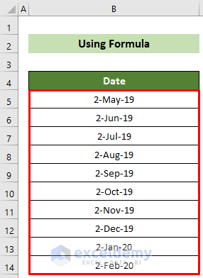
- Drag down the Fill Handle to see the result in the rest of the cells.
This is the output.
Read More: How to Autofill Days of Week Based on Date in Excel
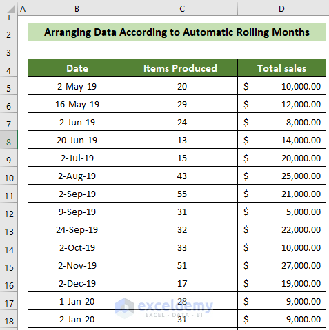
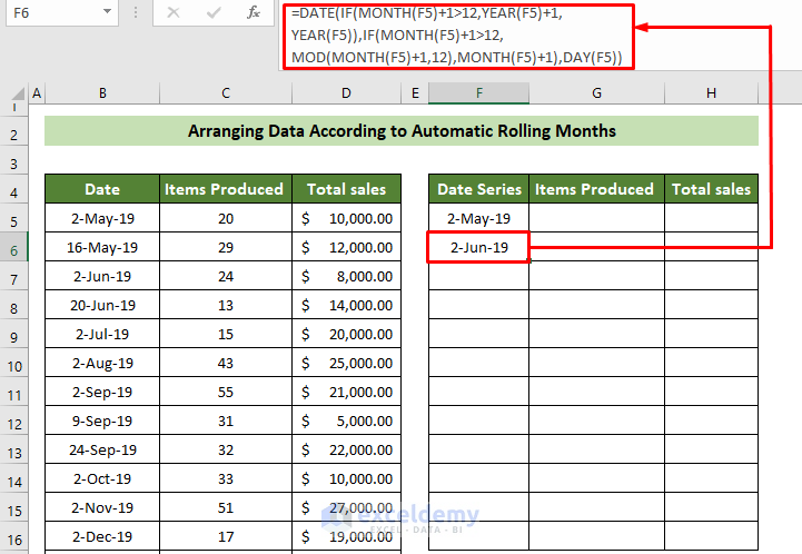
How to Arrange Data According to the Automatic Rolling Months
To find the items produced and sales values for the second date of each month:
Steps:
- Click F5 and enter the starting date.
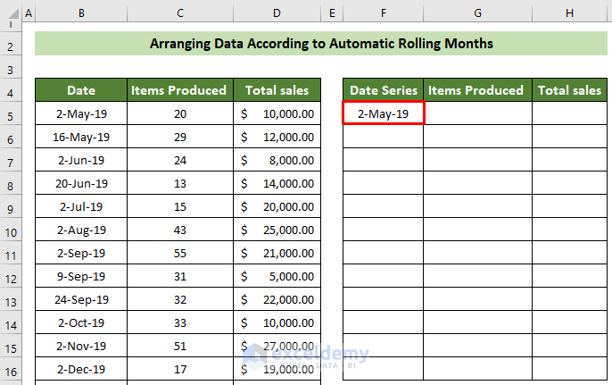
- Click F6 and enter the formula below:
=DATE(IF(MONTH(F5)+1>12,YEAR(F5)+1,YEAR(F5)),IF(MONTH(F5)+1>12,MOD(MONTH(F5)+1,12),MONTH(F5)+1),DAY(F5))- Press Enter.
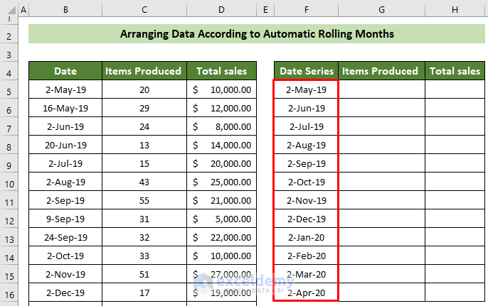
- Drag down the Fill Handle to see the result in the rest of the cells.
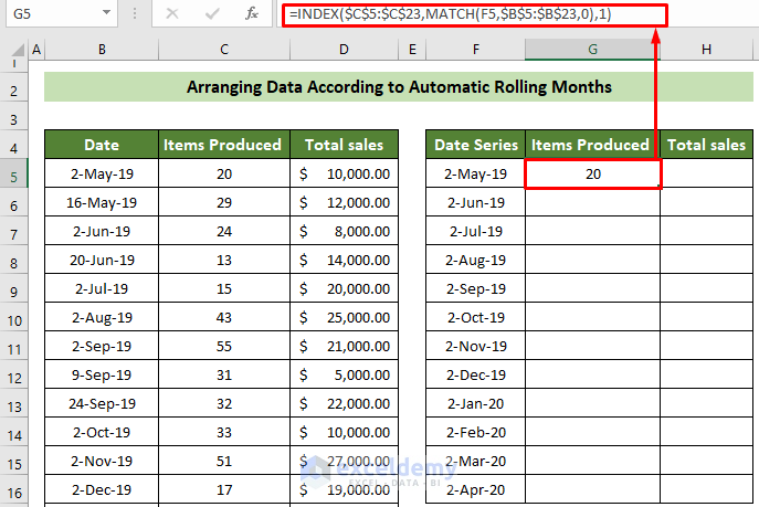
- Click G5 and enter the formula below.
=INDEX($C$5:$C$23,MATCH(F5,$B$5:$B$23,0),1)- Press Enter.
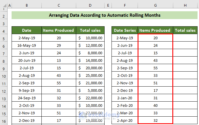
- Drag down the Fill Handle to see the result in the rest of the cells.
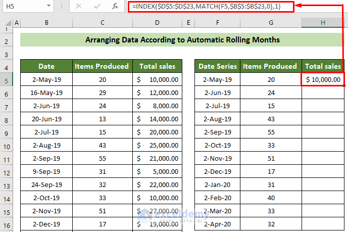
- Click H5 and use the formula below.
=INDEX($D$5:$D$23,MATCH(F5,$B$5:$B$23,0),1)- Press Enter.
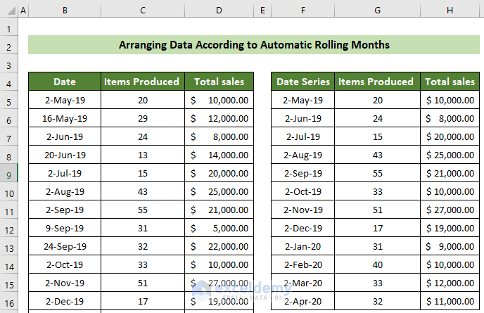
- Drag down the Fill Handle to see the result in the rest of the cells.
This is the output.
Read more: How to Autofill Dates in Excel
Download Practice Workbook
Download the practice workbook.
Related Articles
- Applications of Excel Fill Series
- How to Add Sequence Number by Group in Excel
- How to Increment Month by 1 in Excel
- How to Fill Down Blanks in Excel
- How to Repeat Number Pattern in Excel
- How to Perform Predictive AutoFill in Excel
- How to Enter Sequential Dates Across Multiple Sheets in Excel
<< Go Back to Autofill Dates | Excel Autofill | Learn Excel
Get FREE Advanced Excel Exercises with Solutions!
