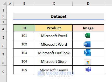
To illustrate how to lock images in a cell, we’re going to use a sample dataset that contains the ID, Product, and Images of the products.
How to Lock an Image in Excel Cell: 2 Methods
Method 1 – Lock an Image in Cell with the Excel Format Picture Feature
Steps:
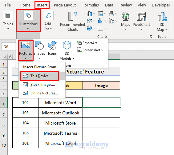
- Go to Insert, select Illustrations, choose Pictures, and pick This Device.
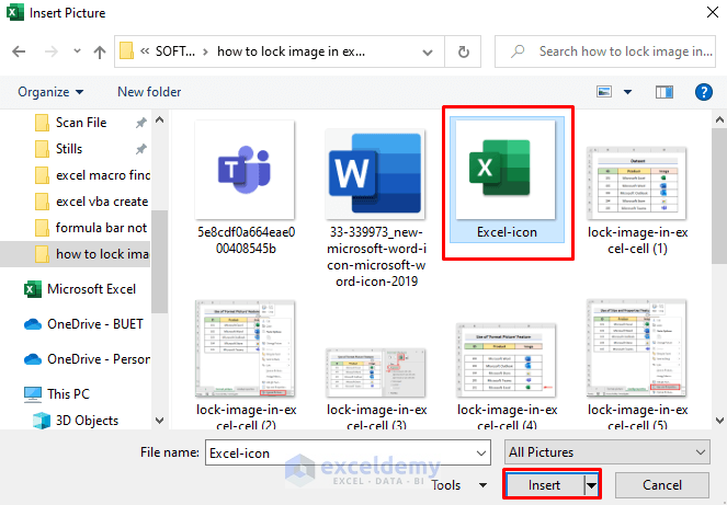
- The Insert Picture window will pop out. Select the picture you want, and press Insert.
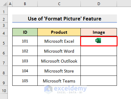
- Resize the picture to fit it in the destination cell.
- Repeat the process to add other images.
- Right-click on a picture to bring up the context menu.
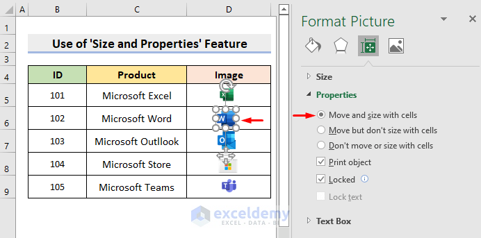
- Choose Format Picture.
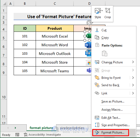
- The Format Picture pane will open up on the right side of the worksheet.
- Under the Size & Properties tab, select Properties.
- Check the circle for Move and size with cells.

- Repeat for other pictures
- Close the Format Picture pane.
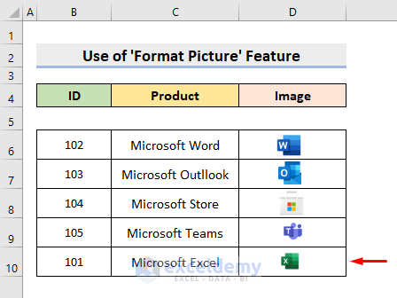
- To see the changes, move row 5 to the 10th row.
- You’ll see the contents of the 5th row now in the 10th row, including the picture.
Read More: How to Link Picture to Cell Value in Excel
Method 2 – Use the Size and Properties Feature to Lock an Image in an Excel Cell
Steps:
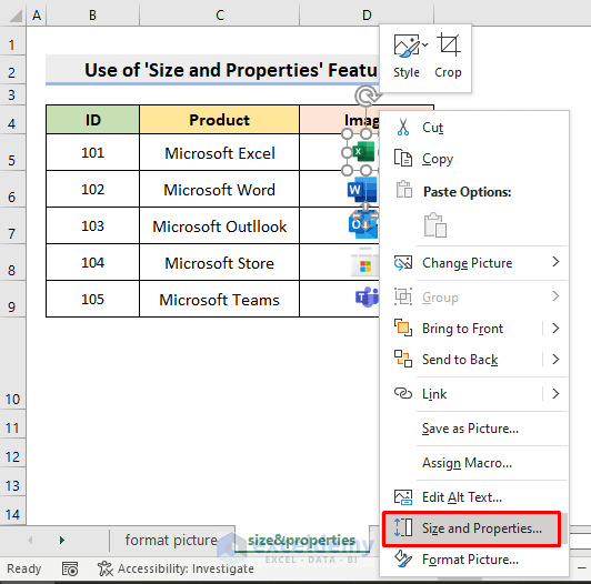
- Select a picture and right-click on it.
- Select Size and Properties.
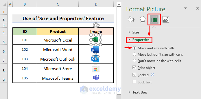
- The Format Picture pane will appear on the right side of the worksheet.
- Check Move and size with cells from Properties.
- Select other pictures and repeat the previous steps.
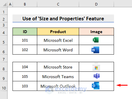
- Close the pane. To observe the changes, move any row.
- In this example, we moved the 7th row. The cell contents of the 7th row including the picture, were moved into the 10th row.
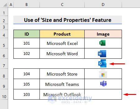
- If we didn’t check the circle for Move and size with cells, the picture would remain where it was. The following picture shows the proof.
Read More: How to Insert Image in Excel Cell as Attachment
Download the Practice Workbook
Related Articles
- How to Insert Picture in Excel Cell Automatically
- How to Insert Pictures Automatically Size to Fit Cells in Excel
- How to Insert Picture in Excel Cell Background
- How to Insert Picture in Excel Cell with Text
- How to Insert a Picture in Excel Header
- How to Insert Multiple Pictures at Once in Excel
- How to Insert Picture in Excel Using Formula
- How to Insert Clipart in Excel
<< Go Back to Excel Insert Pictures | Learn Excel
Get FREE Advanced Excel Exercises with Solutions!

I clicked the “Move and size with cells” circle but when I went to sort my data by a particular column the pictures didnt move with the data. In the Properties menu I have move and size checked and print object checked but nothing else. Please advise.
Hello Kane,
You need to put the picture in one cell. Just resize it and put the image in a single cell then apply the sorting. I think you will get your desired result.
1. First, change the row height of the cell to adjust the image in the cell or resize it to adjust it in a single cell.
2. Then, select the range of cells. Go to the Data tab and select your preferred sorting.
3. Finally, you will see the image is also changing its place while sorting.