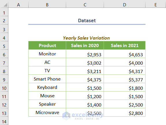
The example dataset below shows the yearly Sales of various Products. The entire dataset is located in the B4:D13 cell range.
Method 1 – Using the Paste Special Option to Get a Linked Picture
In the beginning method, I’ll show you the simple but effective paste options i.e. Linked Picture from the Paste Special option.
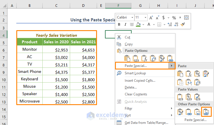
➤ Select the B4:D13 cell range and copy it.
➤ Select any cell where you want to get the linked picture (e.g. F4 cell).
➤ Right-click on the cell where you’d like to get the linked picture. Move the cursor over the rightwards arrow of the Paste Special option and pick Linked Picture under the Other Paste Options feature.
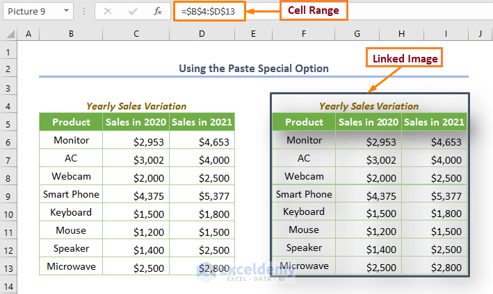
You’ll get a linked picture in the F4 cell as shown in the following screenshot.
NOTE: If you look closely at the formula bar, you’ll see =$B$4:$D$13 which represents the cell values of the Yearly Sales Variation.
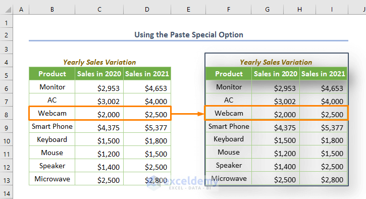
NOTE: This linked picture is not static, which means if you change any value in the original cells you’ll find the changed image. For example, if you input the data of the Webcam product after removing the data of the TV, you’ll get the newly added product in the linked picture.
Read More: How to Insert Picture in Excel Cell Automatically
Method 2 – Using the Camera Tool to Get a Linked Picture
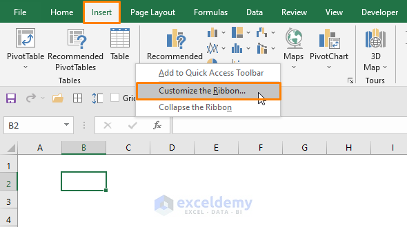
You will probably need to add the Camera tool to your ribbon in Excel because it is not a default tool. To add it, first right-click on the ribbon and choose the Customize the Ribbon option.
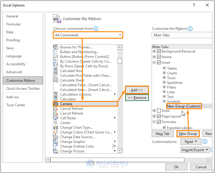
➤ In the dialog box named Excel Options, click on the New Group and create a New Group (Custom).
➤ Click All Commands and find the Camera command.
➤ Click Add.
➤ You’ll see the added command in the Insert tab as shown in the following screenshot.
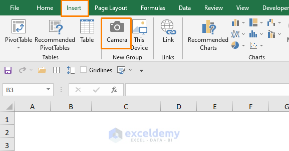
➤ Select the B4:D13 cell range and pick the Camera tool.
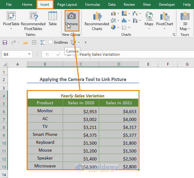
➤ Drag down the cursor following the plus sign located on the right side, as demonstrated in the picture below.
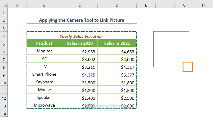
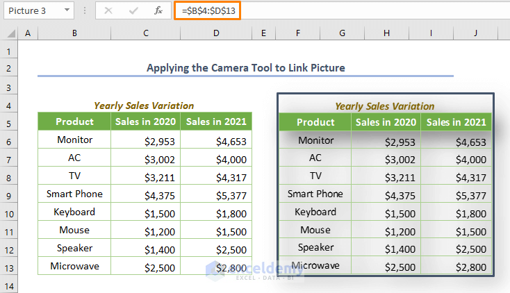
➤ You’ll see the created picture that links with the raw data e.g. Yearly Sales Variation.
Read More: How to Insert Picture in Excel Cell with Text
Method 3 – Using the Hyperlink Option to Get a Linked Picture
Use this method to display the cell value when clicking on an image in your worksheet.
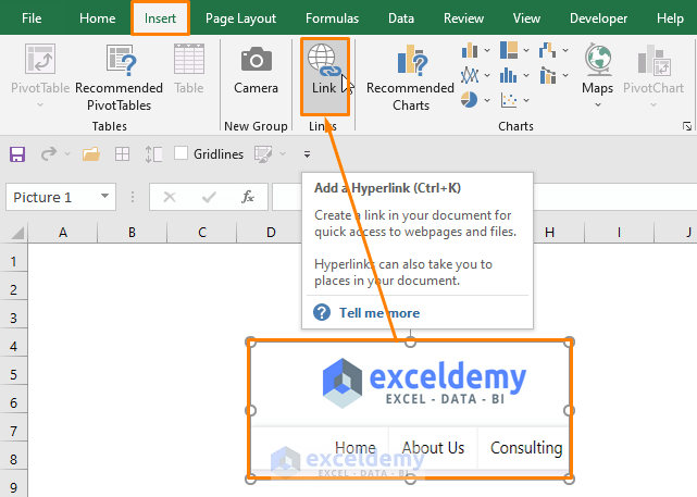
- Select the image

- Choose the Link option from the Insert tab.
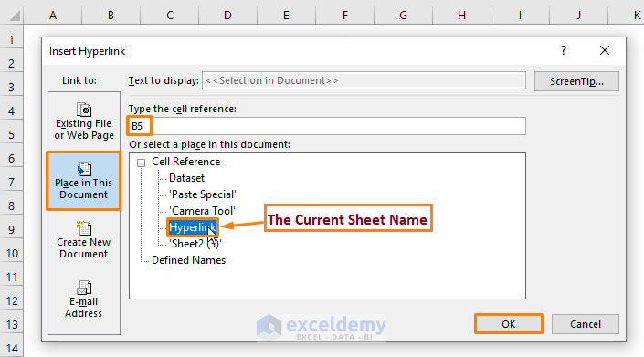
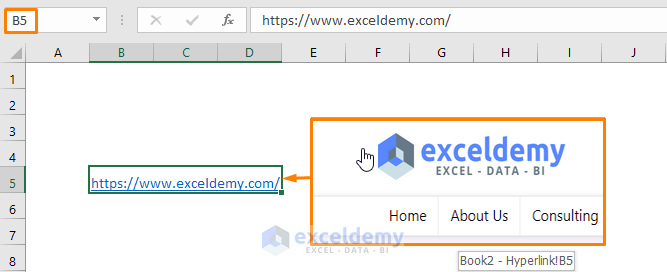
- In the Insert Hyperlink dialogue box, choose the Link to option as Place in This Document. Next, type the cell (e.g. B5) that you want to link in the active working sheet i.e. Hyperlink. Click
- Your existing image is linked with the specified cell. Clicking on the image will display the B5 cell representing the url of ExcelDemy.
Read More: How to Insert Picture in Excel Using Formula
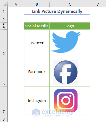
Method 4 – Linking the Picture to the Cell Value Dynamically
This method assumes that you have pictures already saved on your device.
➤ Select a cell.
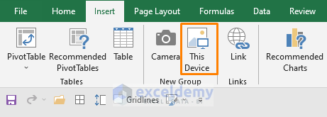
➤ Insert a picture by clicking on the This Device command in the Insert tab of the ribbon. (If this command is not currently on your ribbon, it can be added by using the Customize the Ribbon option as described in Method 3)
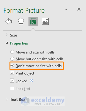
➤ After adding the images, go to the Format Picture option (right-click or go to the right side of your spreadsheet).
➤ Check the circle before the Don’t move or size with cells option.
➤ Adjust the row height and width of the cells to match the size of the picture.
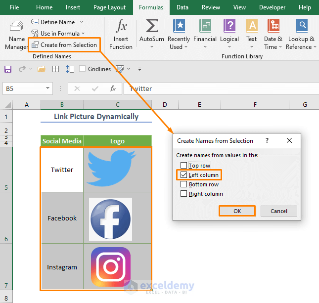
Using the Name Manager tool, you can easily define the names of social media companies with their corresponding logo.
➤ Select the B5:C7 cell range
➤ Click the option Create from Selection in the Defined Names section of the Formulas ribbon. Ensure the box before Left column is checked.
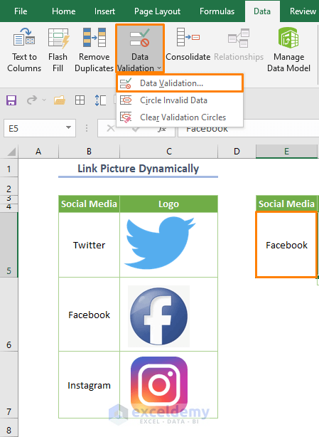
To make the selection more interactive, you can create the drop-down list using the Data Validation tool.
- Choose the Data Validation tool from the Data tab while keeping the cursor over the E5
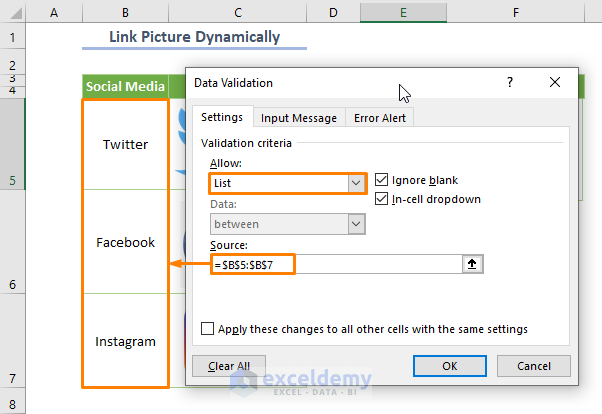
- In the dialogue box, choose List from the drop-down list of the Allow option and set the Source as $B$5:$B$7 and click OK.
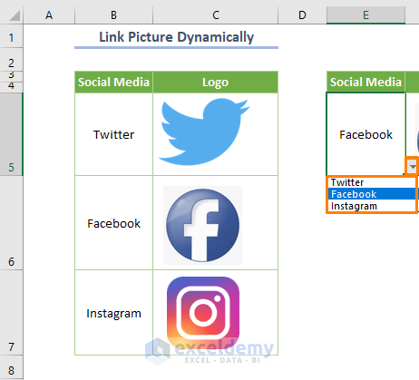
- You’ll get an interactive drop-down list as shown in the below screenshot.
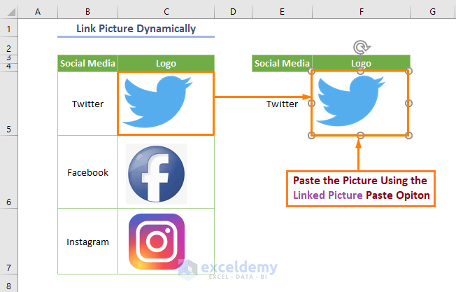
- Paste any picture from the C5:C7 cell range using the Link Picture paste option as shown in the first method. Remember, this picture is not dynamic.
For making the pasted picture dynamic, you need to apply the INDIRECT function which returns the cell values defined by any text string.
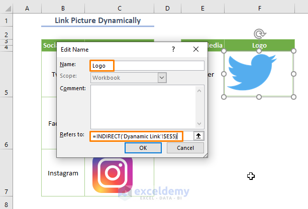
- Open the Name Manager again and click on the New option to create a new defined named range.

- Specify the Name as Logo and insert the following formula in the space after the Refers to
=INDIRECT('Dyanamic Link'!$E$5)(Here, the ‘Dynamic Link’ is the current sheet name and $E$5 is the name of any Social Media.)
- Select the pasted picture and insert the following formula in the formula bar.
=Logo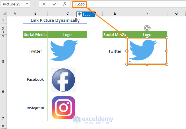
- Your picture is linked dynamically. If you choose any option from Social Media, the picture will be changed automatically.
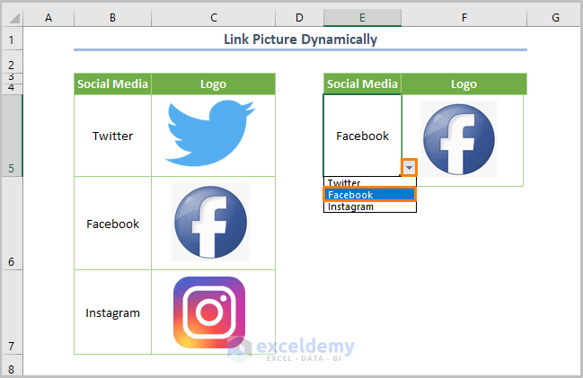
Here, I selected Facebook, and the picture in the F5 cell is changed automatically.
Read More: How to Insert Pictures Automatically Size to Fit Cells in Excel
Download Practice Workbook
Related Articles
- How to Insert Picture in Excel Cell Background
- How to Insert Image in Excel Cell as Attachment
- How to Lock Image in Excel Cell
- How to Insert a Picture in Excel Header
- How to Insert Multiple Pictures at Once in Excel
- How to Insert Clipart in Excel
<< Go Back to Excel Insert Pictures | Learn Excel
Get FREE Advanced Excel Exercises with Solutions!

Your second para doesn’t make sense.
‘Select [this] and select [that].
How do you select two things at the same time?
Hello Frede,
Thank you for pointing that out. The wording in that paragraph was unclear and made it seem like two things needed to be selected at the same time. We’ve updated the article to clarify that the steps should be done sequentially (first select the range, next copy it, then select the destination cell).
We really appreciate your careful reading and helpful feedback!
Regards,
ExcelDemy