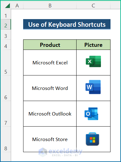
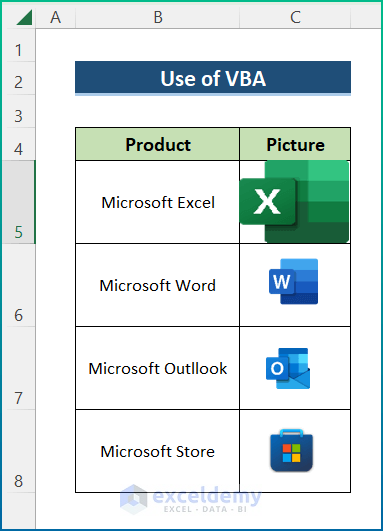
For the purpose of demonstration, I have used the following sample dataset. Here, the dataset contains information about Microsoft Office products. There are 2 columns which, namely the Product and Picture columns.
Method 1 – Utilize Keyboard Shortcuts to Insert Pictures to Fit Cells
Steps:
- Select cell C5.
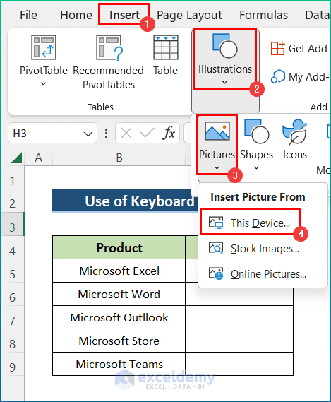
- Go to the Insert tab and click on Illustrations.
- Select Pictures and click on This Device.
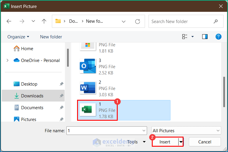
- Select the picture you want to insert from the device where the images are stored and click Insert.
- Similarly, add other pictures as well.
- Adjust the cells according to your desired size.
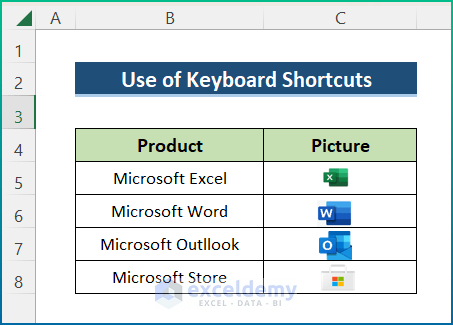
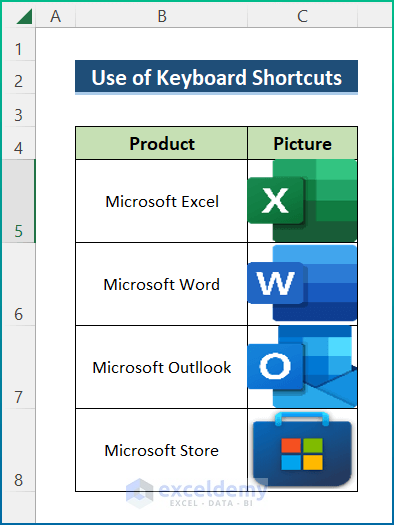
- Hold the Alt key and drag the Microsoft Excel picture until it fits into the cell. Here, the Alt key helps to fit the picture into the entire cell.
- Adjust all the pictures using a similar process.
Read More: How to Insert Picture in Excel Cell Automatically
Method 2 – Using the Format Picture Option in Excel to Make Pictures Fit in Cells
Steps:
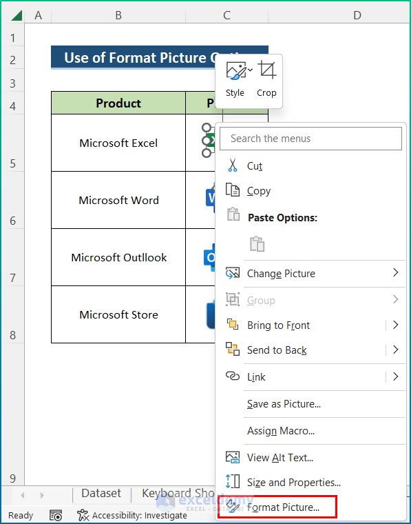
- Select the Excel product picture and right-click.
- Go to Format Picture.
- Select Size and set the Height and Width according to your cell size.
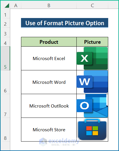
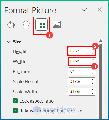 Afterward, the image will fit into the cell.
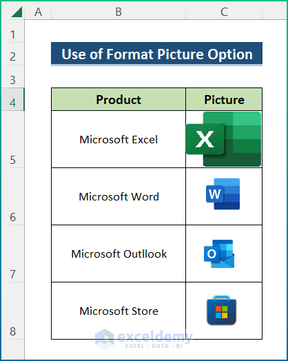
- Similarly, follow the process for the other pictures.
Read More: How to Insert Picture in Excel Using Formula
Method 3 – Inserting Pictures With Excel VBA to Automatically MakeThem Fit in Cells
Steps:
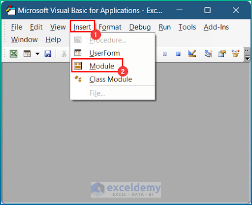
- Hold the Alt + F11 keys in Excel, which opens the Microsoft Visual Basic Applications window.
- Click the Insert button and select Module from the menu to create a module.
- A new window will open. Write the following VBA macro in the Module.
Public Sub AutoResizeImage()
On Error GoTo Select_Image
Dim ZImageWtoHRatio As Single
Dim QWtoHRatio As Single
With Selection
ZImageWtoHRatio = .Width / .Height
End With
With Selection.TopLeftCell
QWtoHRatio = .Width / .RowHeight
End With
Select Case ZImageWtoHRatio / QWtoHRatio
Case Is > 1
With Selection
.Width = .TopLeftCell.Width
.Height = .Width / ZImageWtoHRatio
End With
Case Else
With Selection
.Height = .TopLeftCell.RowHeight
.Width = .Height * ZImageWtoHRatio
End With
End Select
With Selection
.Top = .TopLeftCell.Top
.Left = .TopLeftCell.Left
End With
Exit Sub
Select_Image:
MsgBox "Choose an Image and Run the Macro."
End Sub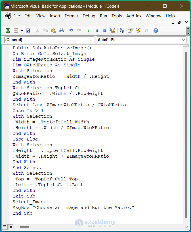
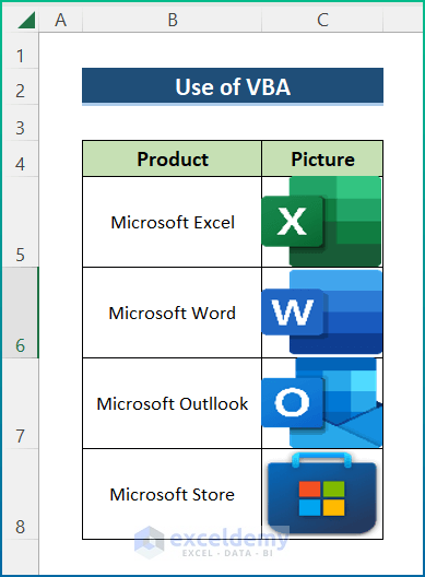
- Select a picture and press the F5 key to run the code.
- Select other pictures one by one and run the code similarly.
Read More: How to Insert Picture in Excel Cell with Text
Download Practice Workbook
You can download the workbook used for the demonstration from the download link below.
Related Articles
- How to Link Picture to Cell Value in Excel
- How to Insert Picture in Excel Cell Background
- How to Insert Image in Excel Cell as Attachment
- How to Insert a Picture in Excel Header
- How to Insert Multiple Pictures at Once in Excel
- How to Insert Clipart in Excel
<< Go Back to Excel Insert Pictures | Learn Excel
Get FREE Advanced Excel Exercises with Solutions!
