The dataset has three columns: Product, Size, and Color.
Method 1 – Utilizing the Insert Tab to Insert a Picture as Cell Background
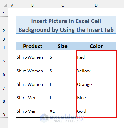
Images will be inserted in the Color column.
Steps:
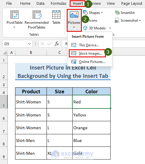
- In the Insert tab >>> Pictures >>> click Stock Images…
Note: If you want to insert images from your device, select This Device… .
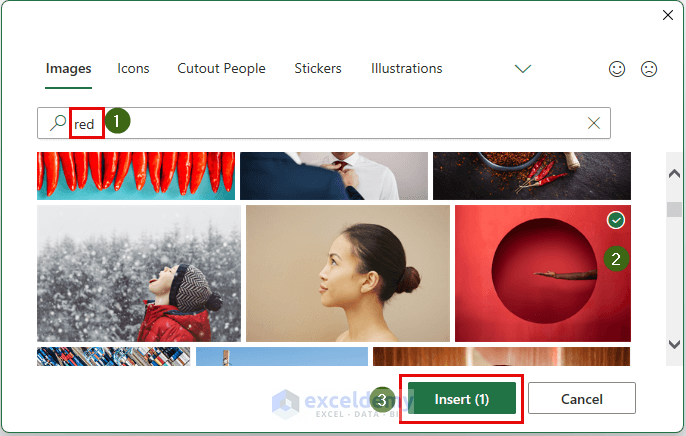
A dialog box will appear.
- Enter a word in the search box, “red”, here.
- Select your image.
- Click Insert.
The selected image will be imported to the worksheet.
- Use the Resize Handles to resize the image and place it in D5.
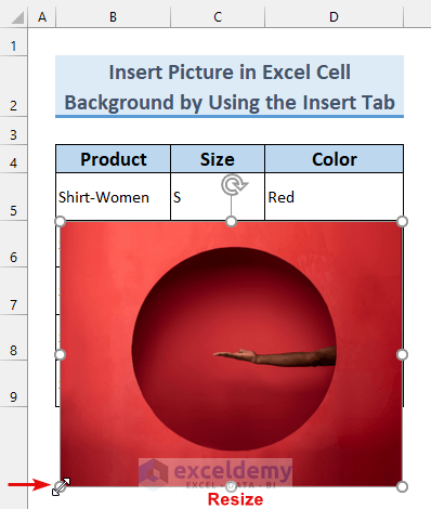
This is will be the result.
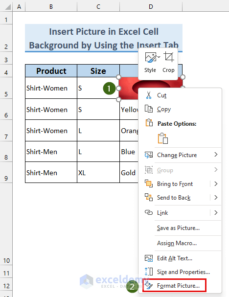
To see the text, increase the transparency value:
- Right-Click the image.
- Click Format Picture…
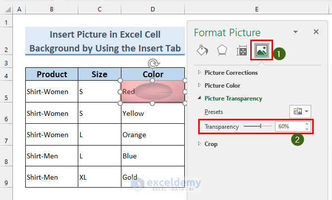
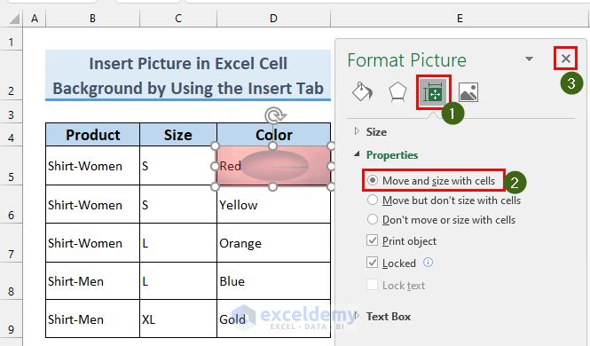
In the Format Picture dialog box:
- Choose Picture >>> Picture Transparency >>> set the Transparency to 60%.
- Go to Size & Properties >>> In Properties select Move and size with cells.
- Close the window.
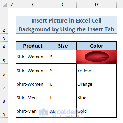
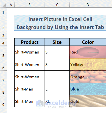
The process can be repeated for other cells.
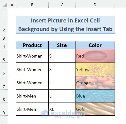
This is the output.
Read More: How to Insert Picture in Excel Cell with Text
2. Using the Page Layout to Insert a Picture in Excel as Cell Background
Steps:
- In the Page Layout tab >>> select Background.
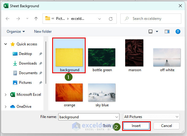
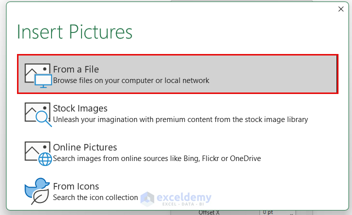
- In the Insert Picture dialog box, select From a file.
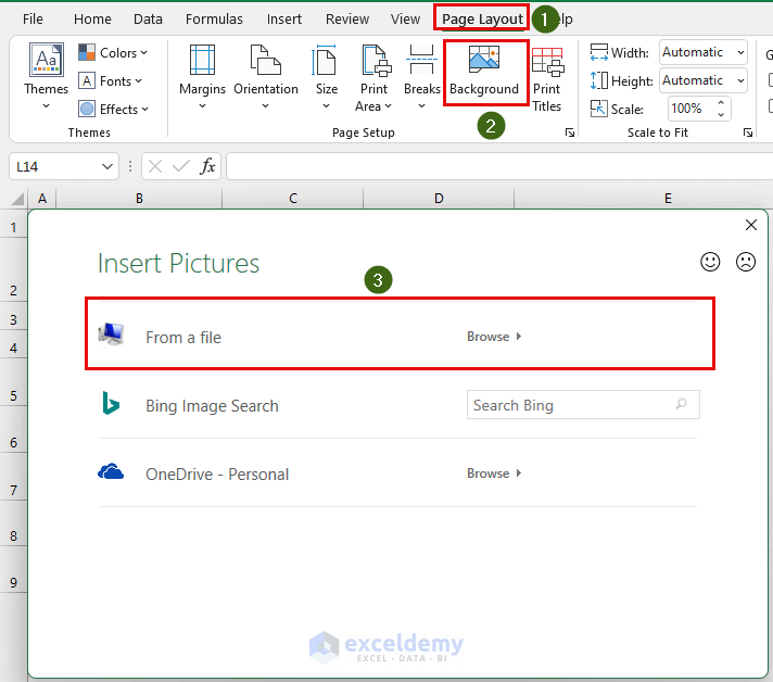
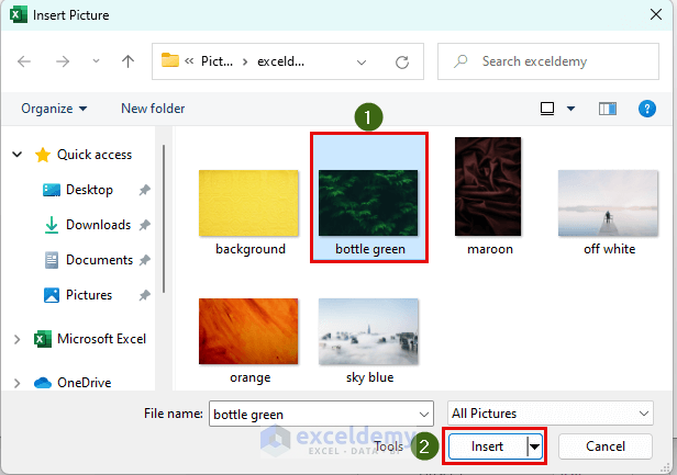
- Select your picture.
- Click Insert.
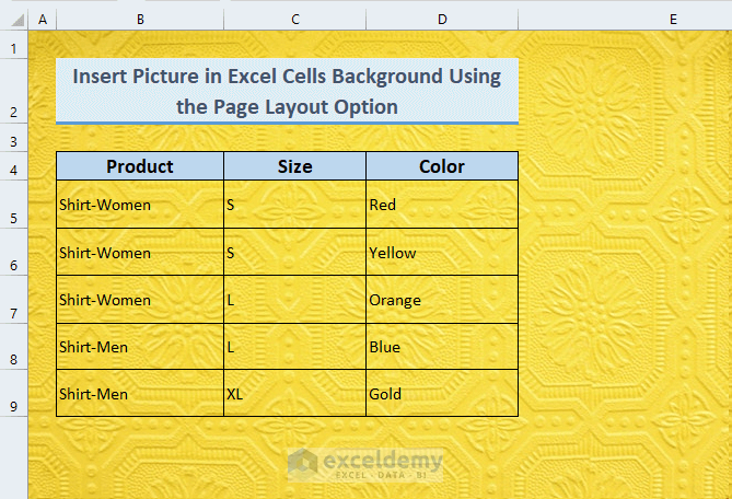
The picture covers the whole worksheet (Photo by Madison Inouye).
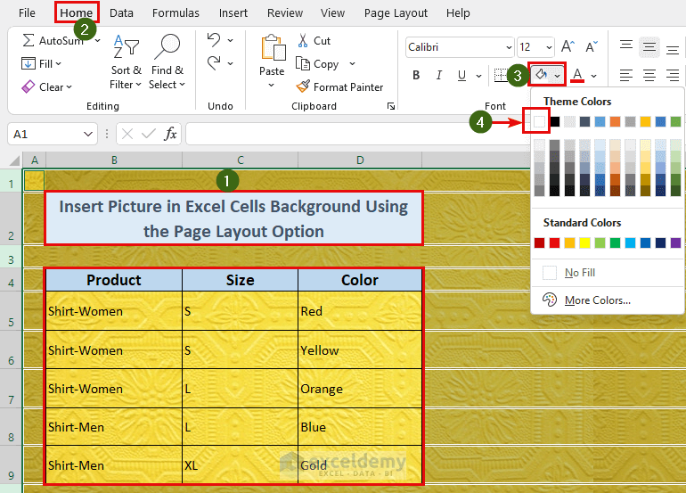
- Select all cells except your dataset.
- In the Home tab >>> Fill Color >>> select White.
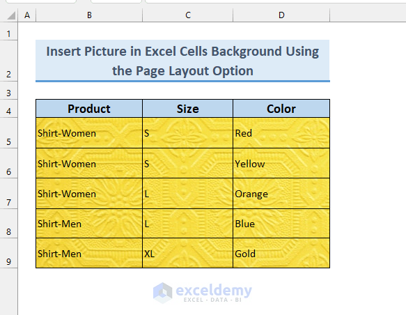
This is the output.
Read More: How to Insert Image in Excel Cell as Attachment
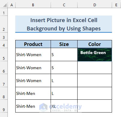
Method 3 – Using the Shape Feature to Insert a Picture in Excel as Cell Background
Steps:
- Go to the Insert tab >>> Shapes >>> select Rectangle.
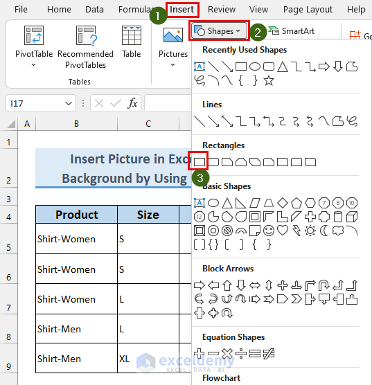
The cursor will be transformed into a plus (+) sign.
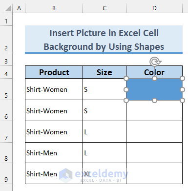
- Draw a rectangle in D5.
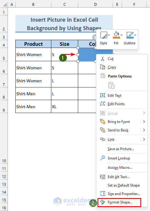
- Right-click the rectangle >>> select Format Shape…
- In Format Picture, choose Fill & Line >>> select Picture or texture fill.
- In Picture source, select Insert… .
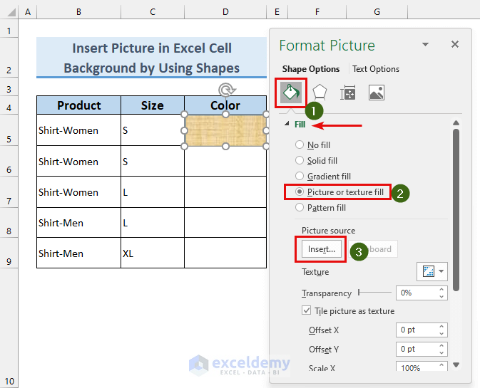
- Click From a File.
- Select a picture.
- Click Insert.
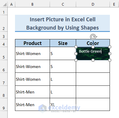
The picture will be displayed in D5.
- Double-click the image to enable write mode.
- Enter your text.
You can change the text style by selecting it.
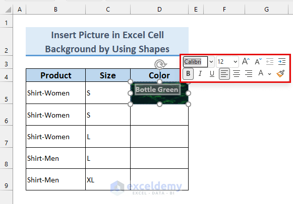
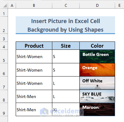
This is the final output.
Repeat the steps to insert pictures as cell background in other cells.
Read More: How to Insert a Picture in Excel Header
Practice Section
Download the file and practice.
Download Practice Workbook
Related Articles
- How to Insert Multiple Pictures at Once in Excel
- How to Insert Picture in Excel Using Formula
- How to Insert Clipart in Excel
- How to Lock Image in Excel Cell
- How to Link Picture to Cell Value in Excel
- How to Insert Picture in Excel Cell Automatically
- How to Insert Pictures Automatically Size to Fit Cells in Excel
<< Go Back to Excel Insert Pictures | Learn Excel
Get FREE Advanced Excel Exercises with Solutions!

Sorry for intrusion but none of solutions combined with the cell itself still the pic. is object and movable and not part of the cell body and change its position and cannot be hidden in case the cell or row belong to it wanted to be…
Hello MAREK,
Hope you are doing well. As far as I understand, you wanted to change the position of the background images or hide any row with these images. I think we can do these works as I demonstrated below.
Firstly, in Section 1, you can move the background image by clicking on the cell and then dragging it to your desired position.
• Here, we have dragged the image beside the cell and changed the text written also in this cell.
• In Section 3, you can move the image along with the text to any position by only clicking on this cell and then dragging it.
In this way, we have changed the position.
• Later, we also changed the text.
• If you want to hide any row, then just click on this row, and then Right-click.
• Select the Hide option.
Eventually, we have hidden our desired row.