How to Insert a Picture in a Cell Automatically – 3 Methods

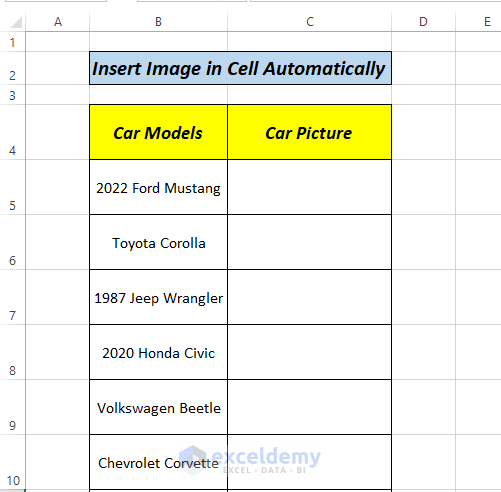
The sample dataset showcases Car Models.

To add pictures:

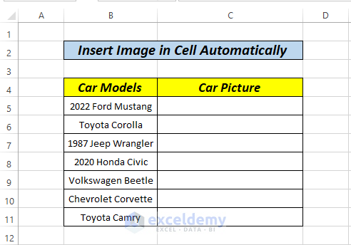
Method 1 – Insert a Picture in an Excel Cell Automatically Using the Insert Tab

Steps:

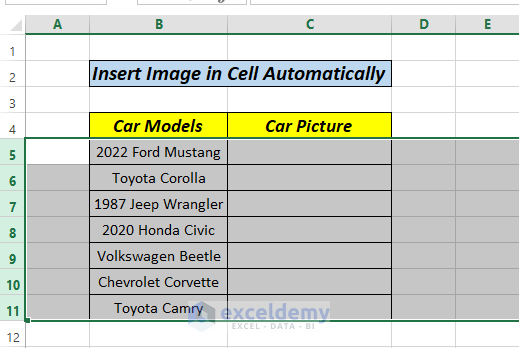
• Adjust the row height. Select the Rows.

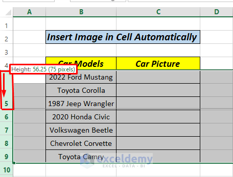
• Drag them down to increase row height.

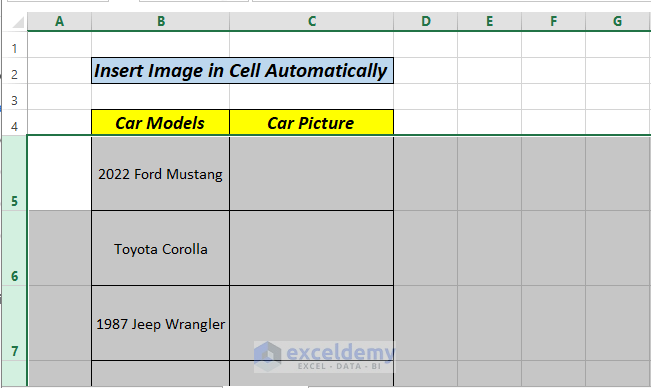
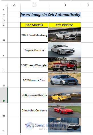
• This is the output.

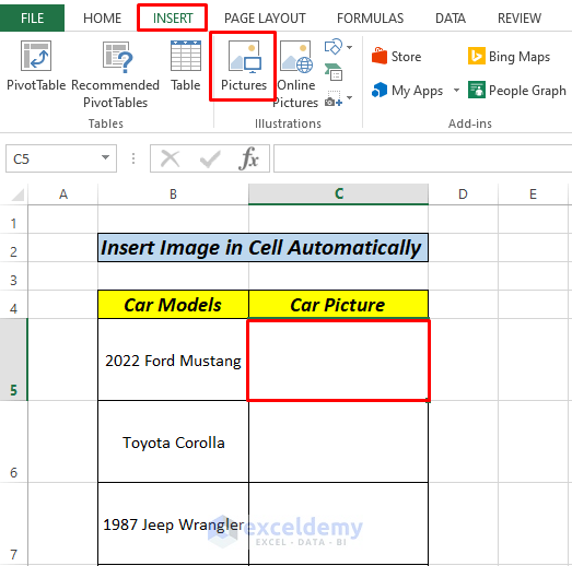
• Click C5 and go to the Insert tab.
• Select Pictures.

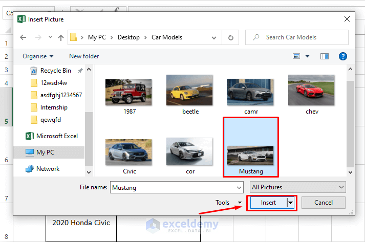
• In the Insert Picture dialog box, choose a folder or drive containing saved pictures.
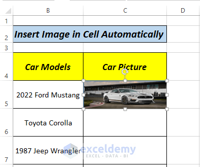
• Select a picture and click Insert.

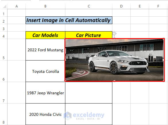
• The image is not in the correct position.

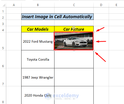
• Hold ALT and resize the image using the corner or side points.

Read More: How to Link Picture to Cell Value in Excel

Method 2 – Using the Shape Fill feature to Insert a Picture in an Excel Cell Automatically

Steps:

• Adjust the row height, as described in Method 1.

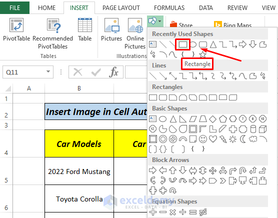
• Go to the Insert tab, select Shapes, and choose Rectangle.

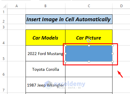
• Draw the shape in C5, as shown below.

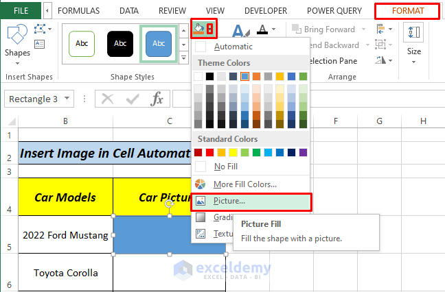
• Go to the Format tab, click the down arrow in Shape Fill.
• Select Pictures as shown below.

• In the dialog box,  choose pictures from a saved file or online. Here, From a File.

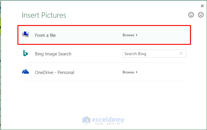
• Select the picture and Insert it.

The image is automatically adjusted to the cell size.

Read More: How to Insert Pictures Automatically Size to Fit Cells in Excel

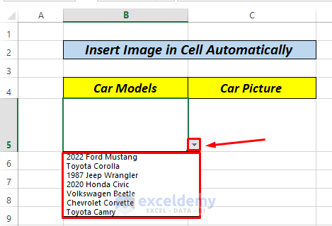
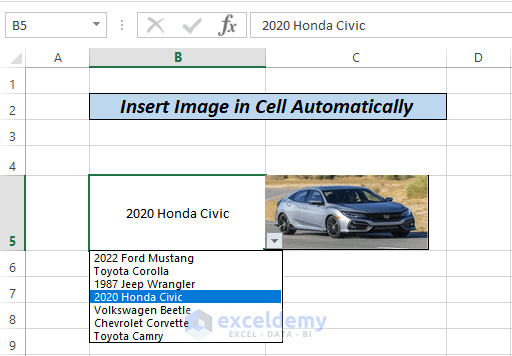
Method 3 – Insert a Picture in an Excel Cell Automatically Using a Dropdown List

Steps:

• Create a list of data and pictures.

• Go to another sheet and select B5.
• Select Data>Data Validation.

• In the dialog box, select List and Range =’Drop Down List’!$B$5:$B$11.

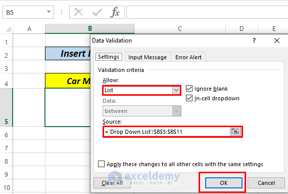
• The drop-down list is created.

• Go to Formulas and select Define Name.

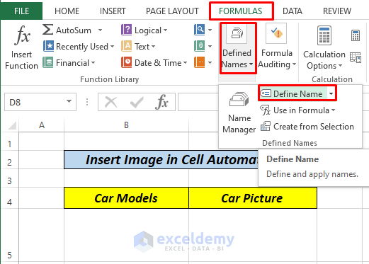
• Define the name as CarLookup and enter the following formula in Refers to.
• Click OK.

$C$5:$C$11 refers to images in the Drop Down List sheet and $B$5:$B$11 refers to the Car Models in the same sheet, and $B$5 is the cell in the Car List sheet.

• Go to the Drop Down List sheet and select the cell behind the image.
• Press CTRL+C.

• In the Car List sheet, select C5 and press CTRL+V.
• Select Linked to Pictures as shown below.

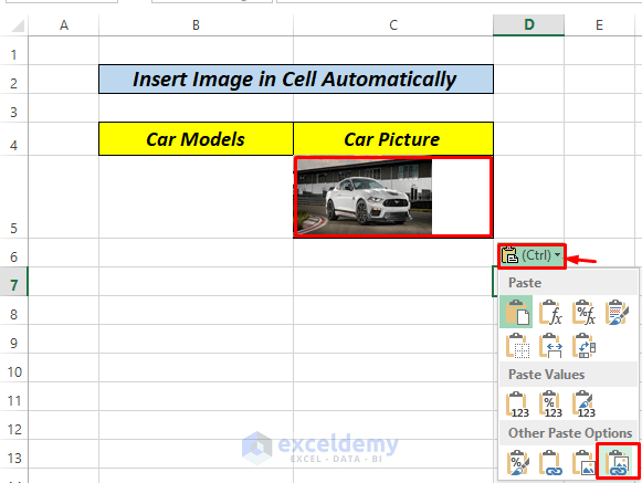
The image is linked.

• Click the Formula bar and enter

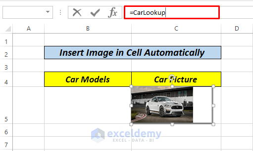
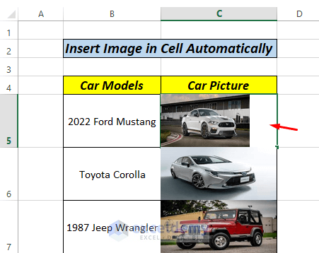
• If you select any car model from the Dropdown List, the image will change automatically.

You can also use XLOOKUP or OFFSET instead of the INDEX function.

Read More: How to Insert Picture in Excel Using Formula

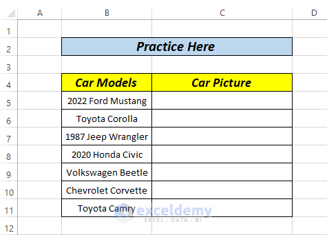
Practice Section

Practice here.

Download Practice Workbook

Related Articles

• How to Insert Picture in Excel Cell Background
• How to Insert Picture in Excel Cell with Text
• How to Insert Image in Excel Cell as Attachment
• How to Lock Image in Excel Cell
• How to Insert a Picture in Excel Header
• How to Insert Multiple Pictures at Once in Excel
• How to Insert Clipart in Excel
  

<< Go Back to Excel Insert Pictures | Learn Excel