How to Insert a Picture in Excel Header

Someone can feel it odd to add pictures in an Excel header. But adding images to a spreadsheet header can be necessary in many cases. When we list products of a company to sell, buyers could like to see the product which can be very useful to impress a buyer. Or maybe you are creating a spreadsheet for your work, and one of the requirements is to include the company logo in the header. It can be tricky if you are not used to doing it. This article will guide you on how to insert a picture to the header in Excel and I hope it will be a simple task for you from now on.

Creating a Header in an Excel Worksheet

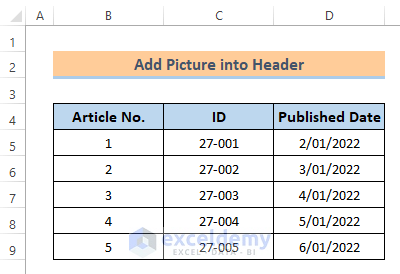
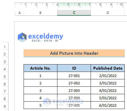
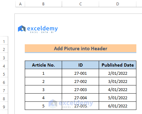
For this article, we’ll use a dataset that represents some data of an online article publisher. Now follow the steps properly to insert a Header in our Excel dataset. If you know how to do it then you can skip this part.

Steps:

• Select the cell where you want to add a Header.
• Then click as follows-

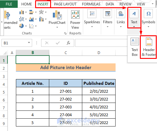
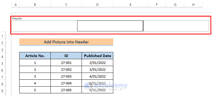
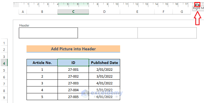
Then the Header will be visible like the image below. Now, look that the header has three boxes.

You can change the alignment of the header from the left and right direction. Press anywhere in the sheet, and you will get the margin. If you keep the mouse in the left margin then you will see an arrow sign like the image below. Click and hold the icon by using the mouse and moving to left or right according to your requirement.

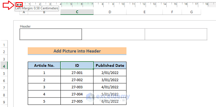
You can change the right margin the same way.

Read More: How to Insert Picture in Excel Cell Background

How to Insert a Picture in an Excel Header

Now let’s go forward to our main task, insert a picture in an Excel Header.

Steps:

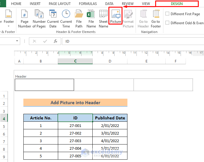
• From the three-part of the Header select the one part where you want to insert a picture.
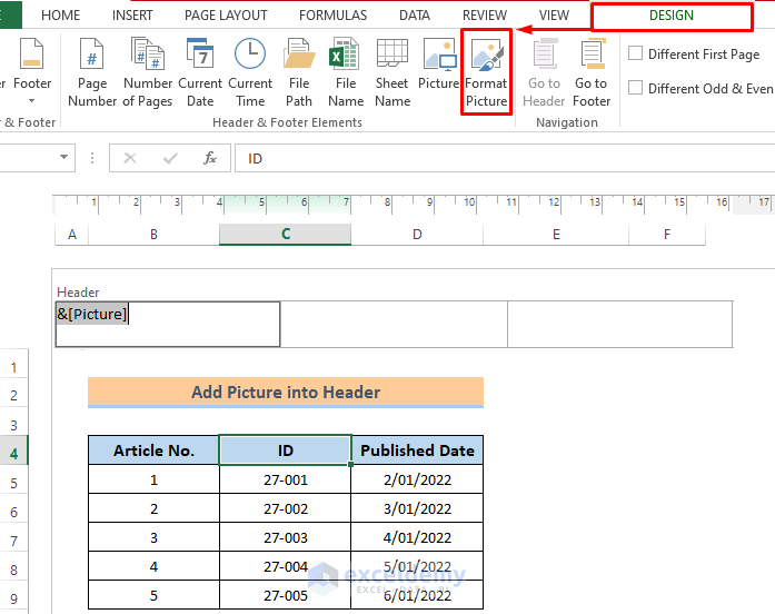
• Then click serially-

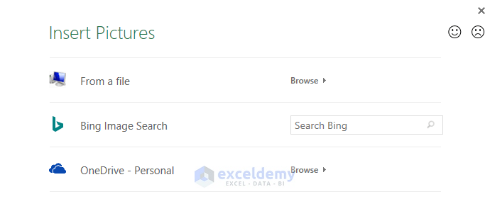
Soon after a dialog box named ‘Insert Pictures’ will appear.

• Select the option where your file is located.
  My file is on my pc so I clicked ‘From a file’.

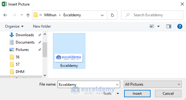
Later, select the image file and press Insert.

After a while, you will observe that there is text into the Header- ‘&[Picture]’. Don’t worry! just press any cell outside of the Header and you will be able to see the image then.

It will look like the image below after adding the picture.

Read More: How to Insert Picture in Excel Cell Automatically

Format the Picture in the Excel Header

Formatting the picture in Excel is pretty different from MS Word or PowerPoint. Here we’ll not be able to resize the picture by dragging the mouse by selecting any corner of the picture rather will have to use a formatting dialog box. Let’s explore that.

Steps:

• Click on the picture by using the mouse.
• Then click as follows-

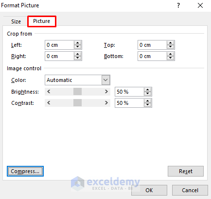
A dialog box named ‘Format Picture’ will open up.

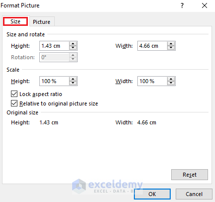
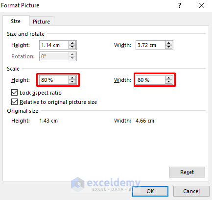
In the Size section, you will get many options to resize the picture like- Rotation, Scaling, etc. You can easily change the height and width of your picture by just putting the required values and then just press OK. Also, there is an option to lock the aspect ratio.

I changed the height and width to 80%.

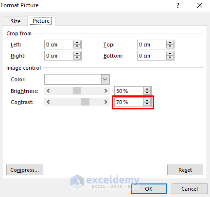
In the Picture section, you can crop the image by putting values relative to the left, right, top, and bottom sides. Besides that, there are options for color grading. You can change the color, brightness, and contrast.

Here, I increased the contrast to 70%. After clicking OK you will get the formatted result.

It’s the formatted output.

Read More: How to Insert Image in Excel Cell as Attachment

Download Practice Workbook

You can download the free Excel template from here and practice on your own.

Conclusion

I hope the procedures described above will be good enough to insert pictures in the Excel header. Feel free to ask any question in the comment section and please give me feedback.

Related Articles

• How to Link Picture to Cell Value in Excel
• How to Insert Pictures Automatically Size to Fit Cells in Excel
• How to Insert Picture in Excel Cell with Text
• How to Lock Image in Excel Cell
• How to Insert Multiple Pictures at Once in Excel
• How to Insert Picture in Excel Using Formula
• How to Insert Clipart in Excel
  

<< Go Back to Excel Insert Pictures | Learn Excel