In this Excel tutorial, we will discuss how to apply different types of alignment in Excel. We will use different techniques like using control text options and the Format Cells dialog box to apply different types of alignment. We will also explain how to change alignment in Excel, and how to align numbers based on a custom number format as well as by using functions.
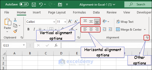
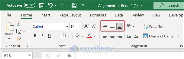
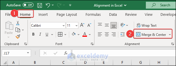
In the following image, we display how to change the alignment from the ribbon. There are vertical and horizontal alignment options, along with Orientation, Indentation, Wrap Text, and Merge & Center options. All the other options are available if you click on the marked arrow in the bottom-right corner of the Alignment group .
Download Practice Workbook
What Is Alignment in Excel?
Generally, alignment refers to the arrangement and positioning of elements within a document. In Excel, it refers to the positioning of cell contents within a cell. To customize the appearance and layout of data in cells, there are various types of alignments available in Excel, like Horizontal alignment, Vertical alignment, Text Orientation, and so on. Combining these alignment options, we can make data easily understandable and more visually organized in Excel.
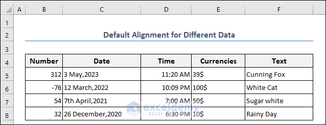
The default alignment for numbers and text is different in Excel. For example, the default alignment of number, date, time, and currencies is the right bottom alignment, while the text has the left bottom alignment. The following image shows the different default alignments for different data types.
What Are the Excel Alignment Options and How to Use Them?
Method 1 – Horizontal and Vertical Alignment Options
The two main alignment options in Excel are the horizontal and vertical alignments of text. Each has three different alignment options.
1.1 – Horizontal Alignment of Cells in Excel
I – Left Alignment
To apply the Left alignment to cells, select them first. Then choose the left align option as shown in the following image.
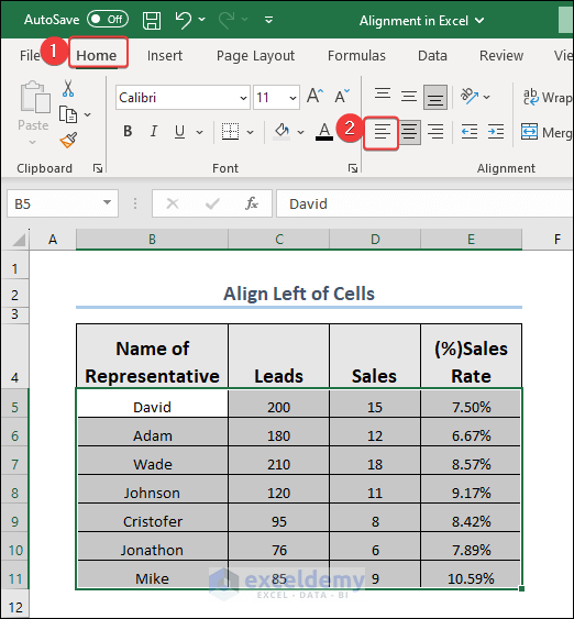
The selected cells will look like the image below.

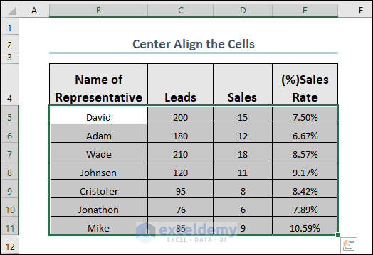
II – Center Alignment
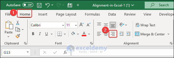
To apply the Center horizontal alignment, select the cell or your desired area and click on the ribbon like in the following image.
The selected cells will look like the image below.
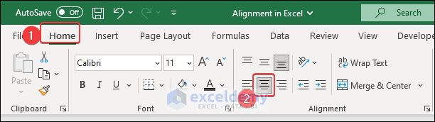
III – Right Alignment
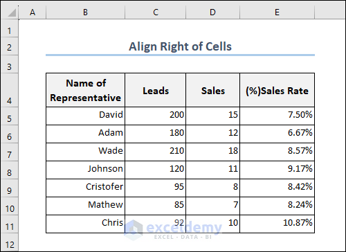
The third type of horizontal alignment is Align Right. Like in the methods described above, select the text to which you want to apply this alignment, then follow the steps shown in the following image.
The selected data will look like the following image.
1.2 – Vertical Alignment of Cells
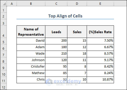
I – Top Alignment
To position the text or content in the upper part of a cell, choose Top Align. Choose the Top option in the Vertical: drop-down menu of the Format Cells dialog box.
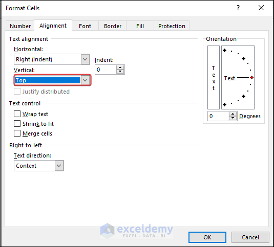
The output of this alignment looks like the following image.
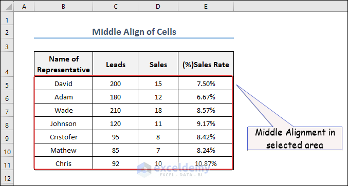
II – Middle Alignment
To apply Middle Align to your cell contents, select the cell first, then follow the steps in the image below.
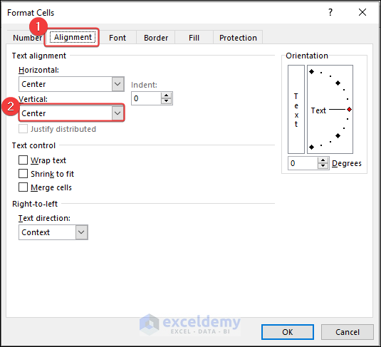
The selected area will look like the image below.
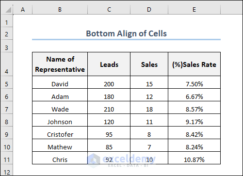
III – Bottom Alignment
The last type of vertical alignment is Bottom Align. The image below shows how to apply bottom alignment in cells.
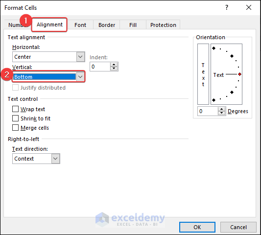
The output looks like the following image.
Method 2 – Changing Text Orientation
We can easily change the text orientation using the Format Cells dialog box.
- Select the text for which you want to change the orientation and press Ctrl+1.

Click to see the full view of image
- Change the Degrees under the Orientation tab and provide a suitable value.
For example, by placing 82 in the Degrees box, the output is as in the image below.

Read More: All Types of Alignment in Excel
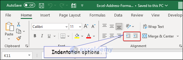
Method 3 – Changing Indentation
Indentation in Excel is the increase or decrease of space between the left and right margin of a paragraph. There are 2 options available in Excel by which you can increase or decrease the indentation of text.
3.1 – Increase Indentation of Texts
- Select the data for which you want to change the orientation.
- Go to the Home tab, and in the Alignment group click on Increase Indent
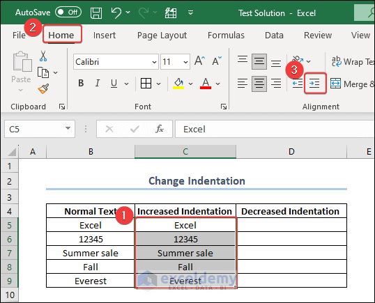
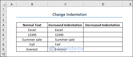
The first output will be like the following image.
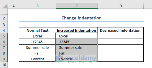
- Increase the indentation further, and the output will be as follows:
Method 4 – Wrapping Text to See Very Long Text in Multiple Lines
When the text in a cell is very long, Excel has some problems accommodating it. The text may expand to the next cell, or it may be difficult to read the contents. We can use Wrap Text to solve the issue.
- Select the cell to wrap, then select Wrap Text under the Home tab.
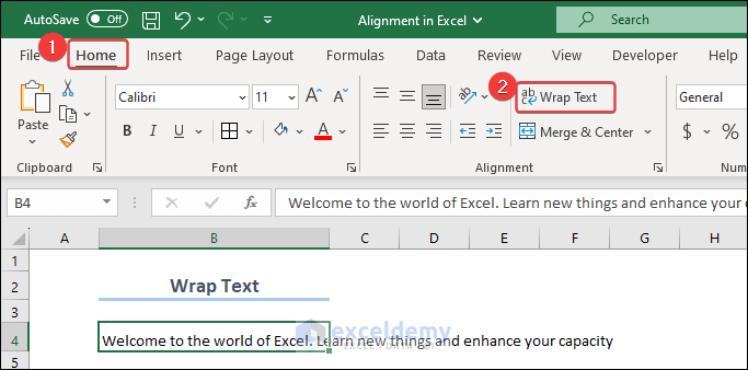
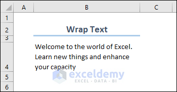
The output will be like the following image.
Read More: How to Align Text in Excel
Method 5 – Using the Merge and Center Command
To combine multiple cells into one, choose the Merge & Center option in the Home tab.
Read More: How to Middle Align in Excel
More Alignment Options Available in the Format Cells Dialog Window
Option 1 – Justify Mode in Horizontal Alignment
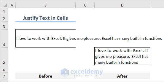
Justification gives text a cleaner and more formal look by adding white space between the words in each line so that all the lines are the same length.
To apply the Justify tool to your text:
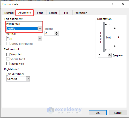
- Select the text and press Ctrl+1 to open the Format Cells dialog box.
- Under the Alignment tab, change the option for Horizontal: Justify then click OK.
In the following image is the output before and after applying Justify alignment to a certain text.
Read More: Justify Text in Excel
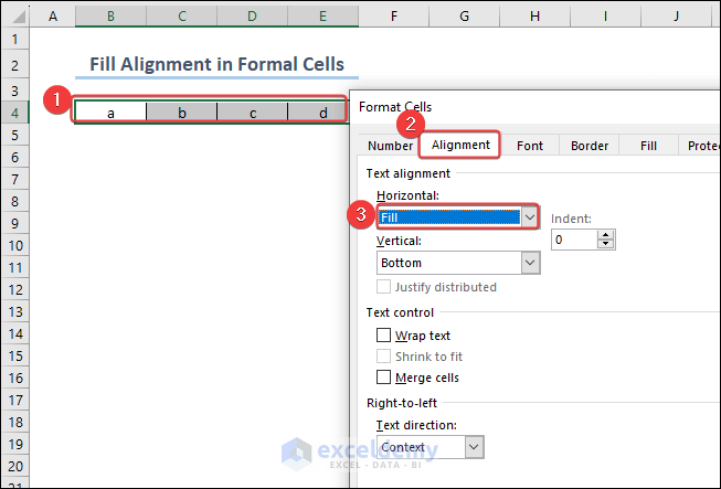
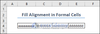
Option 2 – Filling a Whole Cell with the Current Content
Suppose you need to write the same letter in a cell multiple times. To automate this tiresome job, use the Fill feature.
- Select where you want to apply the Fill
- Press Ctrl+1 to open the Format Cells dialog box.
- Select the options as follows:
The cell will be filled with the same letter
Option 3 – Using the Shrink to Fit Command
Another way to represent large text in a single cell is using Shrink to Fit.
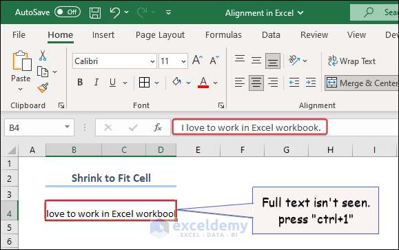
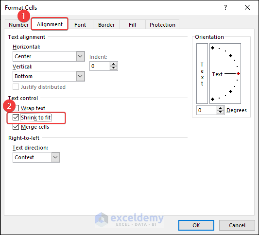
- Select the cell and press Ctrl+1 to open the Format Cells dialog box.
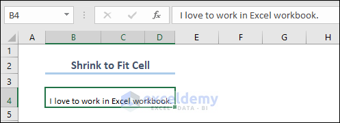
- Choose the following options in the dialog box:
The output will be like the following image.
Option 4 – Using the Center Across Selection Command
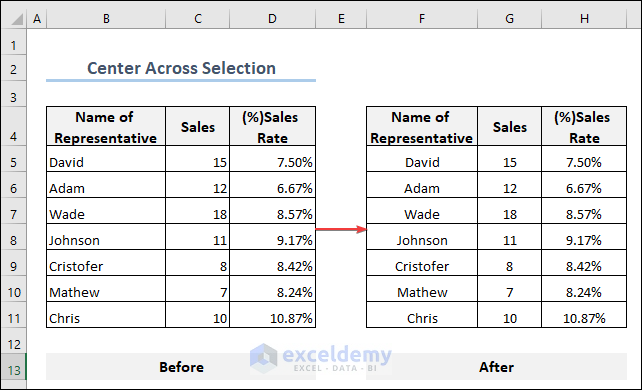
The Center Across Selection command aligns the content of any cell centrally. Suppose we have a dataset where all the cells contain different values that have default alignment. We will change the alignment into Center Across Selection.
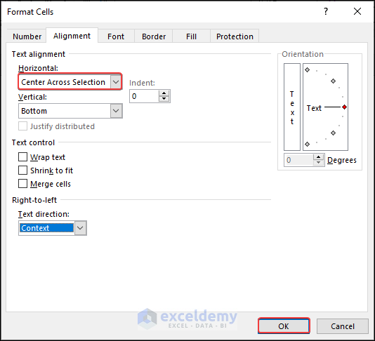
- Select the data and open the Format Cells dialog box.
- In the Horizontal: drop-down menu, select Center Across Selection.
The following image illustrates Center Across Selection alignment.
Read More: How to Center Text in a Cell in Excel
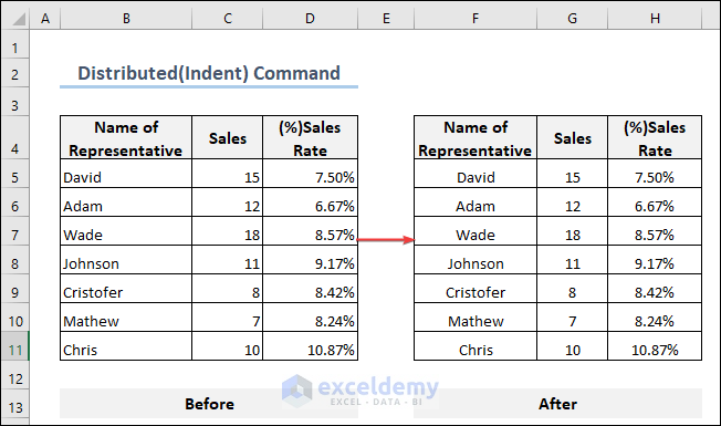
Option 5 – Using the Distributed (Indent) Command
The last Horizontal alignment that we will cover is Distributed (Indent). The process is exactly the same as using the Center Across Selection command. Just select the Distributed (Indent) command in the Horizontal: drop-down option instead of the Center Across Selection command.

The output will be similar to the following image.
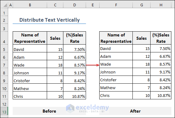
Option 6 – Distributing Text Vertically
To distribute text vertically:
- Open the Format Cells dialog box.
- Choose the Distributed option in the Vertical: drop-down menu.
The output will look like the image below.
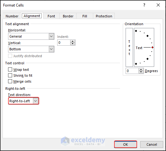
Option 7 – Using the Right-to-Left Option to Change the Text Reading Direction
This option is dedicated to those languages that have default right-to-left reading directions like Arabic. Applying this feature to other languages is not possible. However, in the following image is the method to change the default orientation using the Format Cells dialog box.
Keyboard Shortcuts for Alignment in Excel
There are keyboard shortcuts for most of the methods described above:
| Name of Alignment | Shortcut Keys |
|---|---|
| Align Left | ALT + H + A + L |
| Center | ALT + H + A + C |
| Align Right | ALT + H + A + R |
| Top Align | ALT + H + A + T |
| Middle Align | ALT + H + A + M |
| Bottom Align | ALT + H + A + B |
How to Revert to the Default Alignment of Cells
Reverting to default alignments of cells is a simple task.
Steps:
- Click on the cell or cells that you want to revert to their default alignment.
- Press Ctrl+1 to open the Format Cells dialog box.
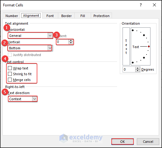
- Choose the Alignment tab.
- In the Horizontal: drop-down box, select General.
- In the Vertical: drop-down box, select Bottom.
- Set “0” as the Indent.
- Uncheck all the boxes under the Text Control options.
- Set Text Direction to Context.
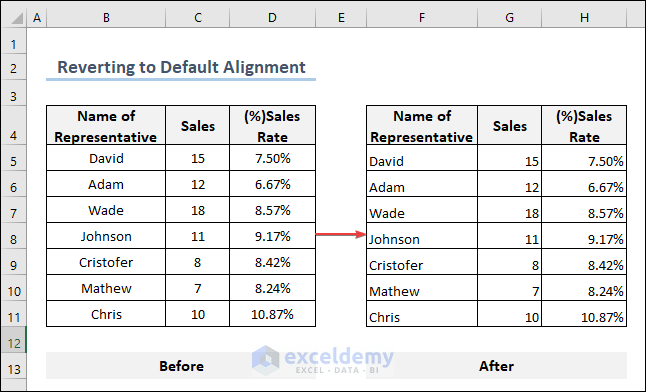
To illustrate, suppose we have a dataset where the data is in a different alignment to the default alignment. Here’s how it looks before and after being reset into default alignment.
How to Change the Alignment of a Number Using a Custom Format
First step is to open the Custom Number Format option:
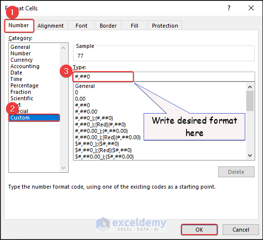
- Select the column that contains numbers, and open Format Cells.
- Under the Number tab, select as follows:
In the image below, we have a dataset that contains different numbers. We will format and align the numbers using the custom number format.
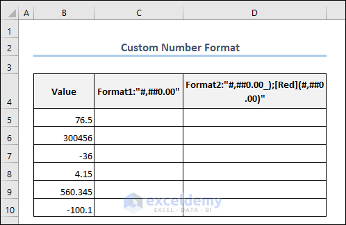
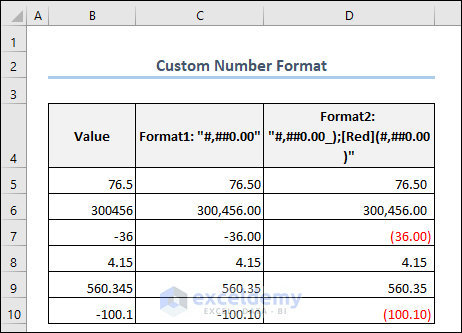
- In Column C, apply the following format to the numbers:
#,##0.00- In Column D, we’ll apply different formatting. The formula is as follows:
#,##0.00_);[Red](#,##0.00)The result of applying these two formats will be similar to the following image.
Read More: How to Align Numbers in Excel
Things to Remember
- Maintain consistency throughout the workbook.
- Use merged cells only when it is really necessary, since the process discards all the data except for that in the first cell.
- Utilize the Wrap Text feature when the contents of cells are to long to fit within the cell borders.
- Preview and adjust the alignment to optimize the printed appearance.
Frequently Asked Questions
1. How can I align the content in merged cells to ensure consistency across the merged area?
Answer: Alignment for merged cells is identical to normal cells. Apply horizontal and vertical alignment and ensure consistency of the content in the merged cell.
2. Can I apply conditional formatting based on the alignment of cell contents in Excel?
Answer: No, you cannot directly apply conditional formatting based on the alignment of cells. Conditional formatting does not have the built-in functionality to consider the alignment of cells.
3. What is the difference between “Merge Cells” and “Center Across Selection” for aligning content across multiple cells?
Answer: Merge Cells combines selected cells into one cell, discarding content from other cells, whereas Center Across Selection horizontally centers content across selected cells without merging them, maintaining separate cells.
Alignment in Excel: Knowledge Hub
<< Go Back to Excel Cell Format | Learn Excel

