When you enter any number in the Excel worksheet cell, you will see the number will align on the right side of the cell as a default. This is a normal procedure in Excel. In this article, we will discuss the details of the default alignment of numbers in Excel. I hope you find this article interesting and useful for your future purposes.
What Is Alignment in Excel?
Alignment can be defined as the position of your text or number in a cell. In Microsoft Excel, you can align your text or number vertically and horizontally. In the case of horizontal alignment, you can align your text or number on the left, center, or right side of the cell. Whereas, in terms of vertical alignment, you can align your text or number on the top, middle, or bottom side of the cell. But Microsoft Excel has its default alignment options. For any text, it will align on the left side of the cell and at the bottom of it. Moreover, when you enter any number, it will align on the bottom right corner of the cell as a default.
How Many Alignments Are Available in Excel
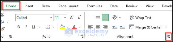
In Microsoft Excel, there are basically two types of alignments: vertical and horizontal. Both of them are divided into several more types. To get the alignment types, you need to go to the Home tab on the ribbon. Then, click on the Small Tilted Arrow at the bottom of the Alignment group.
In the Format Cells dialog box, you will get those two types of alignments. From there, you can choose the alignment that you would like to have in a cell.
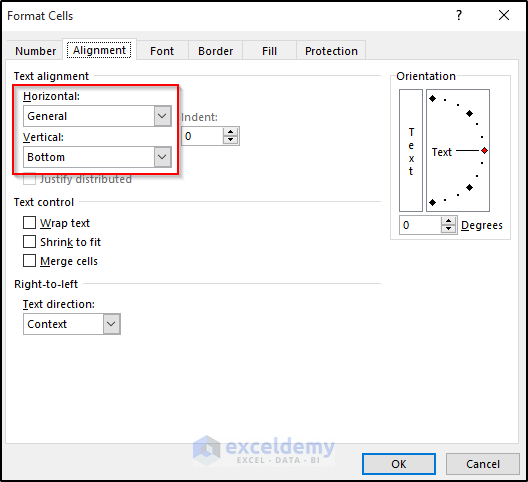
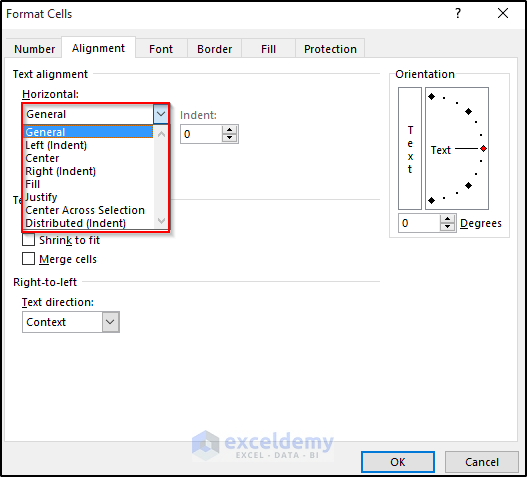
When it comes to horizontal alignment, you have so many options such as left alignment, center alignment, or right alignment. But by default, Excel will provide left alignment for text and right alignment for numbers.
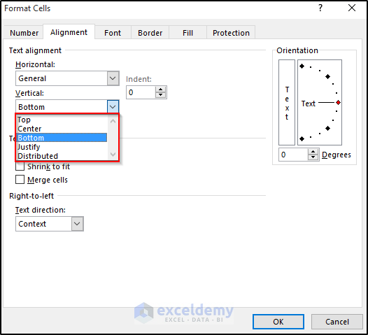
Whereas, in terms of vertical alignment, you can align your text or number on the top, middle, or bottom side of the cell.
Read More: All Types of Alignment in Excel
What Is the Default Alignment of Numbers in Excel?
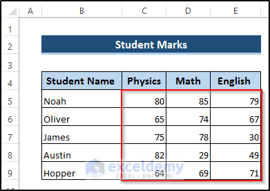
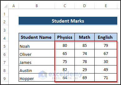
In Microsoft Excel, the default alignment of numbers is on the bottom right side of the cell. When you enter any number in your worksheet, you will see the default alignment automatically. But you can alter this by changing the vertical and horizontal alignment. It is totally your own call. In Microsoft Excel, they will provide you with a default alignment for entering any number or text. Here, we take a dataset that includes student marks. Now, when we insert any marks, it is aligned on the bottom-right side of the cell.
How to Change Default Alignment of Numbers in Excel
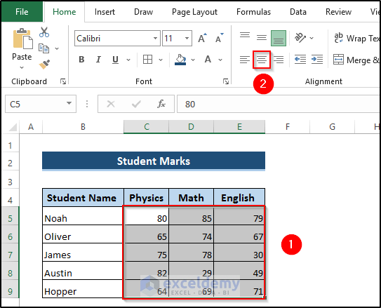
After entering any number on the Excel worksheet, you will see the default alignment. The Excel puts the number on the bottom right side of the cell. But you can easily change horizontally or vertically according to your wish. In the dataset, first, select the cells having numbers. Now, go to the Home tab on the ribbon. Then, from the Alignment group, select the Center Align option.
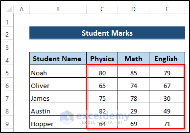
As a result, you will see all the numbers are aligned centrally.
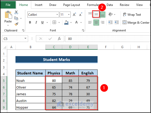
Next, in terms of vertical alignment, Excel puts numbers at the bottom of the cell. If you want to change the vertical alignment, then, first go to the Home tab on the ribbon. Then, select the Middle or Top Align option from the Alignment group. Here, we select the Middle Align option.
As a consequence, we will see the following change because of the vertical alignment in the cells.
Read More: How to Change Alignment in Excel
What Is the Alignment of Text and Formula in Excel?
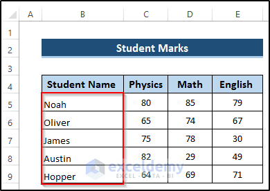
The alignment of the text can be divided into two types: horizontal and vertical. Horizontally, the default alignment of text is on the left side of the cell. Whereas, the default vertical alignment of text is at the bottom of the cell. Here, look at the dataset where we include text in a cell.
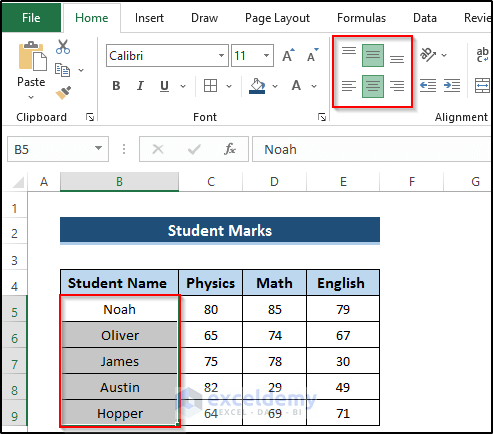
Now, you can change the alignment both horizontally and vertically. To do this, first, select the cells having text. After that, go to the Home tab on the ribbon. Then, select any of the horizontal and vertical alignment options from the Alignment group.

Here, we use the center and middle alignment. As a result, we get the following alignment. See the screenshot.
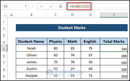
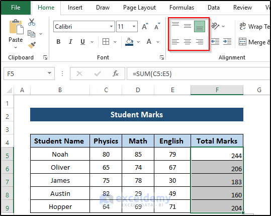
Now, when we add a formula to a cell, the default alignment will be on the right side of the cell and also at the bottom end.
But, you can change the alignment like the previous one. Here, select the cell with the formula. Then, go to the Home tab on the ribbon. After that, select any alignment from the Alignment group.
Here, we use the center and middle alignment. As a result, we get the following alignment. See the screenshot.

Read More: How to Align Text in Excel
Download Practice Workbook
Download the practice workbook below.
Conclusion
We have shown the details of the default alignment of numbers in Excel. In this article, we have also included how to change the default alignment of numbers in Excel. After going through the article, I think you have a clear idea of default alignment. If you have further questions, feel free to ask in the comment box.
Related Articles
- How to Align Colon in Excel
- How to Align Decimal Points in Excel
- How to Center Text in a Cell in Excel
- How to Align Columns in Excel
- How to Justify Text in Excel
- How to Align Currency Symbol in Excel
- How to Align Numbers in Excel
<< Go Back to Alignment in Excel | Excel Cell Format | Learn Excel
Get FREE Advanced Excel Exercises with Solutions!
