How to Change Alignment in Excel (5 Easy Methods)

We often face trouble while changing alignment according to our needs in Excel. If you are facing the same, this tutorial will show you 5 different methods to change alignment in Excel with steps.

5 Easy Methods to Change Alignment in Excel

Aligning text or numbers is a property of formatting that affects how a paragraph of text looks. Here, we’ll talk about all five ways, with steps and proper explanations.

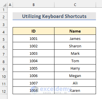
In this tutorial, we’ll use the dataset below, which has the ID and Name of each student in a class. The dataset is set up so that text and numbers are aligned by default in Excel so that you can understand it better.

1. Using Excel Ribbon to Change Alignment in Excel

We will start with the easiest and Excel-provided options from Ribbon to change the alignment in Excel. To do so, we will follow the steps below.

Steps:

• First, we need to select all the data we need to change alignment. In our case, it’s from B4 to C12.

• Second, we will go to Ribbon and in the Home tab, find the Alignment Here we will find the following options.

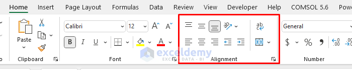
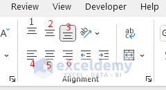
• Here we have multiple options for alignment such as Top Align(1), Middle Align(2), and Bottom Align(3) to choose for vertical alignment. And for horizontal alignment, we have Align Left(4), Center(5), and Align Right(6). By default, the alignment is Bottom Left for texts and Bottom Right for numbers as we saw in the reference dataset.

• Third, we need to select the alignment according to our needs. Here is an example where we have selected Center and Middle alignment.

Read More: How to Left Align in Excel

2. Alter Alignment in Excel with Custom Number Format

The Custom number format is another way to change the text alignment in Excel. It requires some advanced knowledge of Excel string representation. Here is a step-by-step procedure for this method.

Steps:

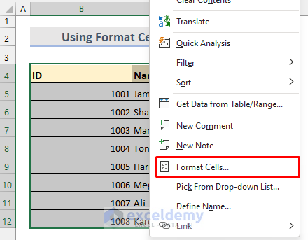
• Firstly, we need to select all the cells where we want to change alignment. In our case, the cells are B4 to C12 and then right-click on it. We will have various options. Among them select the Format Cells option.

• Secondly, selecting this option will open a panel like the following image. In the panel, find Custom at the bottom of the panel.

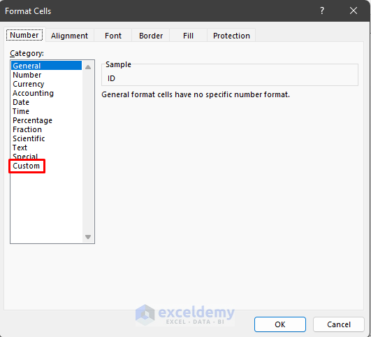
• Thirdly, going to the Custom option, we can write our text pattern under the Type Section.

• For example, we want to right assign all our texts. So we will type * @ in the text field Type.
• Here the * sign means the empty space of a cell. The @ sign indicates the start of the string.

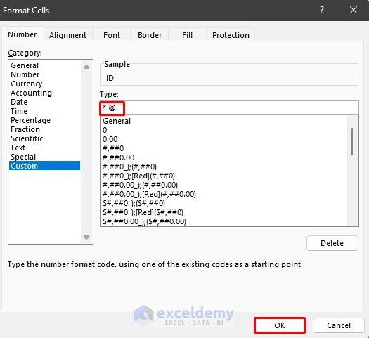
• Finally, after pressing ok we will see all our texts of selected cells are right aligned.

Read More: How to Align Right in Excel

3. Utilizing Keyboard Shortcuts

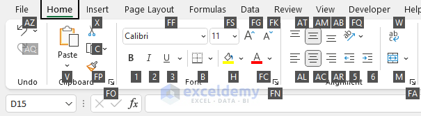
For fast and advanced typing, we can utilize keyboard shortcuts to change the alignment of texts and numbers in Excel. Different alignments have different keys assigned to them. We can see those keyboard shortcuts by pressing ALT+H. It’ll show the Home tab like this:

To change the alignment of text as before, we will follow these steps.
Steps:

• At first, we need to select the data cells as before.
• Then we will press ALT+H to activate the Home tab.

• Next, we need to change the alignment. For example, we want to get our text in the center both vertically and horizontally. To do so we will press A+M for taking the texts vertically center.

• Lastly, to change horizontal alignment, again we need to press ALT+H. Then we will press A+C. Following those steps, we can get the following result.

Read More: How to Apply Center Horizontal Alignment in Excel

4. Change Alignment in Excel Using Format Cells Dialog Box

We can also change alignment in Excel using the Format Cells dialog which is also a built-in option in Excel. Here are the steps to change alignment using it.

Steps:

• In the beginning, all the steps are the same. We will select the data and then we can press CTRL+1 to open the Format Cells
• Next, we will search for Alignment in the Format Cells panel.

• Then we can select the vertical and horizontal positioning from the Text Alignment Here we can choose different alignments. As we did in the earlier example, we will bring our texts to the center both vertically and horizontally.

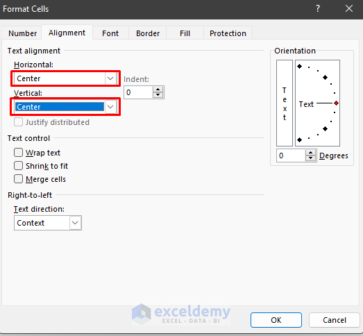
• Finally, by pressing OK, we will get our expected result like the image below.

Similar Readings

• All Types of Alignment in Excel
• How to Top Align in Excel
• How to Middle Align in Excel
• How to Bottom Align in Excel
• Align Decimal Points in Excel

5. Applying VBA Code to Change Alignment in Excel

We can apply VBA to develop our custom macro functions to do the same work as well. To do so, we need to follow these steps.

Steps:

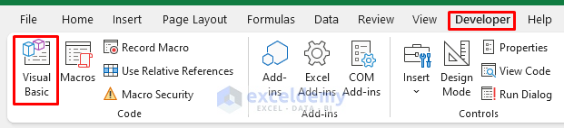
• First, we need to go to the Developer tab in the ribbon and click on Visual Basic.

• Next clicking this will open a new window. In that window, select Insert and then click on Module.

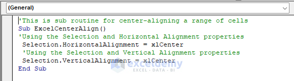
• In the writing area, write the code of the image below and then exit the panel.

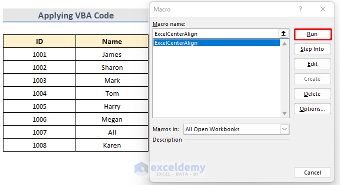
• Finally, after selecting the cells, we want to change, choose Macros in the Developer That will give us a panel like this. In the panel click on Run and we will get our expected output.

Things to Remember

• Changing Alignment will always show the changes in the Ribbon.
• By using the Number Format, we can not change vertical alignment.
• For any keyboard shortcuts, we need to trigger the Home tab first by clicking ALT+H.
• Before running VBA, we need to select the range of cells we want to modify.

Download Practice Workbook

You can download the practice workbook from here.

Conclusion

Changing alignment is often used in Excel to visually modify or create a structure of any file. Hope this article will help you to do so. If you’re still having trouble with any of these methods, let us know in the comments. Our team is ready to answer all of your questions.