In many cases, you might need to align cells to the left in Excel. It is very easy to choose or change alignment in Microsoft Excel. Also, you can do this kind of task in bulk within seconds in Microsoft Excel. This article demonstrates how to align left in Excel with three handy methods.
How to Left Align in Excel: 3 Easy Ways
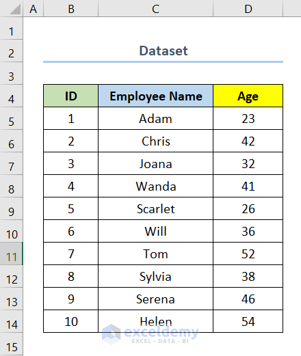
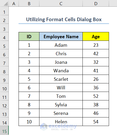
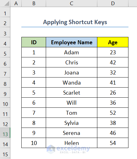
Let’s assume you have a dataset where you have the list of a number of employees with their ID and Age. In this dataset, the cells for the columns ID, Employee Name, and Age contain an alignment of center. At this point, you want to change their alignment to the left. In the following stages of this article, we will see three methods to do so.
We have used the Microsoft Excel 365 version here, you can use any other version according to your convenience.
1. Using Standard Toolbar to Left Align in Excel
In this method, we will use the Standard Toolbar in the Home tab to align the contents of the following dataset to the left in Excel. This is a very simple and fast procedure. Now, follow the below steps to do so.
Steps:
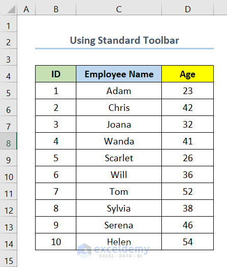
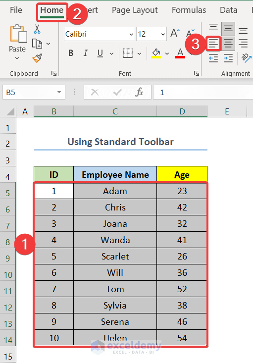
- At the very beginning, select range B5:D14.
Here cells B5 and D14 are the first and last cells of the columns ID and Age respectively.
- Next, go to the Home tab.
- After that, from the Alignment options select Align Left.
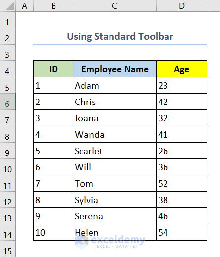
- Eventually, you will have an output like the screenshot below where all the cells now contain a left alignment.
Read More: How to Align Text in Excel
2. Utilizing Format Cells Dialog Box
Now, in this method, we will use the Format Cells Dialog Box to left align. This method is very convenient when you want to apply a lot of change at once. At this point, follow the below steps to align the contents to the left utilizing the Format Cell Dialog Box.
Steps:
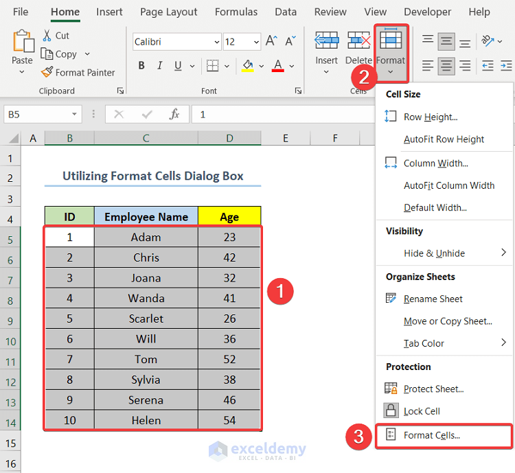
- First, select the range B5:D14.
- Next, go to Format from the Home tab.
- After that, select Format Cells.
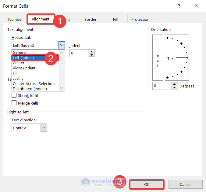
Afterward, the Format Cells dialog box will pop up.
- Now, go to Alignment.
- Then from the Text Alignment Horizontal options select Left (indent).
- Consequently, click on OK.
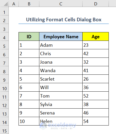
- Finally, you will have your cells left aligned as shown in the below screenshot.
3. Applying Shortcut Keys to Left Align
The fastest way to left align is to use the shortcut keys. Now, to left align in Excel apply the shortcut keys, and follow the below steps.
Steps:
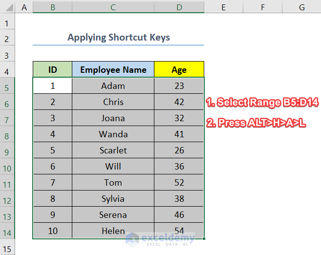
- In the beginning, select range B5:D14.
- Next, press ALT > H > A > L.
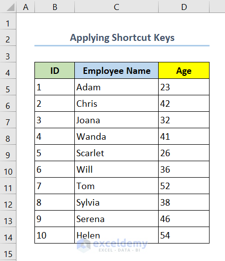
- Eventually, you will have your output as shown in the below screenshot.
Read More: How to Center Text in a Cell in Excel
Download Practice Workbook
You can download the practice workbook from the link below.
Conclusion
In this article, I have shown you three different methods to left align in Excel. You can use any of these three methods to left align. Also, you can use these methods to change to other alignments just by adopting some little changes to these methods.
Last but not least, I hope you found what you were looking for in this article. If you have any queries, please drop a comment below.
Related Articles
- How to Change Alignment in Excel
- [Fixed!] Excel Cell Alignment Not Working
- All Types of Alignment in Excel
- How to Top Align in Excel
- How to Middle Align in Excel
- Align Two Sets of Data in Excel
- How to Bottom Align in Excel
- How to Align Right in Excel
- How to Apply Center Horizontal Alignment in Excel
<< Go Back to Alignment in Excel | Excel Cell Format | Learn Excel
Get FREE Advanced Excel Exercises with Solutions!
