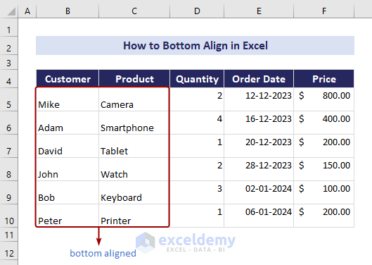
How to Bottom Align in Excel (3 Easy Ways)

The dataset below contains both texts and numbers, where the texts are vertically bottom-aligned and the numbers are top-aligned.

Method 1 – Using the Bottom Align Command from the Alignment Group

Select the cells you want to align vertically at the bottom. We have selected the range B5:C10.
Go to the Home tab on the Excel Ribbon.
In the Alignment group, select the Bottom Align icon.

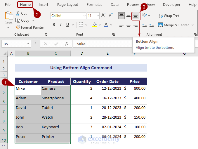
In the image below, you can see that Excel has aligned the selected range vertically in the bottom position of the cell.

Note: To bottom-align in Excel, you can use a keyboard shortcut. Select the desired cells and press Alt + H + A + B.

Method 2 – Using the Format Cells Dialog Box

Select the range of cells.
Right-click on them.
From the context menu, choose the Format Cells command.

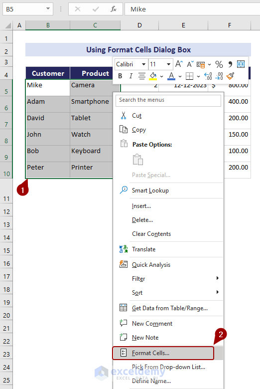
The Format Cells dialog box will appear.

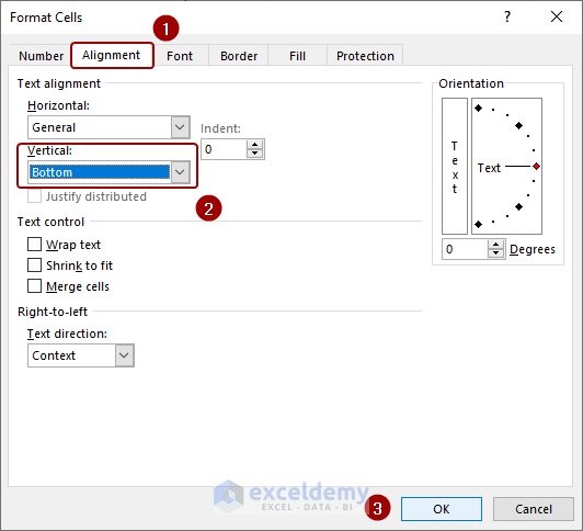
Go to the Alignment tab and the Text alignment group.
Choose the Vertical drop-down and select Bottom.
Hit OK.

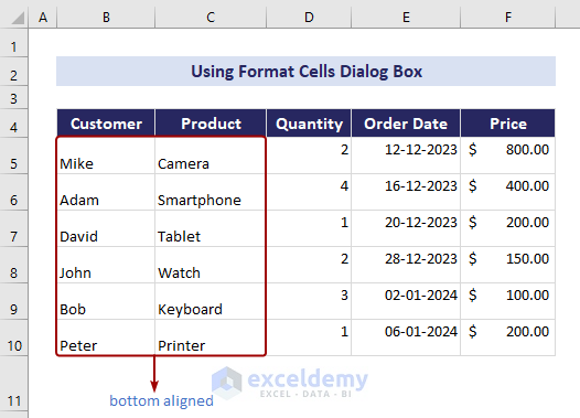
Excel will bottom-align your cell content. We have selected the range B5:C10 to make it bottom-aligned.

Note: You can also launch the Format Cells dialog box by pressing Ctrl + 1 or clicking the Alignment Settings arrow in the Alignment group of the Home tab.

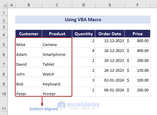
Method 3 – Using VBA Macro

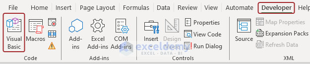
Go to the Developer tab and select Visual Basic. Alternatively, press Alt + F11.
The “Microsoft Visual Basic for Applications” window will appear.
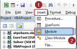
Click Insert and select Module.

Insert the following code in the Module:

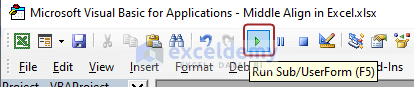
Sub bottom_alignment()
'Specifying the range for bottom alignment
Range("B5:C10").VerticalAlignment = xlBottom
End Sub

Click Run to execute the VBA macro.
Excel will bottom-align the specified range in the VBA code. As we specified the range “B5:C10” in the code, Excel has adjusted the alignment of this range vertically in the bottom position of the cell.

Read More: How to Align Numbers in Excel

Download the Practice Workbook

How to bottom Align in Excel.xlsm

Frequently Asked Questions

Why does Excel default to bottom alignment?

Excel defaults to bottom alignment for text and numbers to maintain a clean and consistent appearance. As the bottom alignment leaves space above the cell border, you can easily navigate to the end of the content in a cell. Besides, as the aim of inventing Excel was to ease calculations, it drew inspiration from traditional accounting practices, particularly old accounting books.