Top alignment in Excel refers to showing the content at the uppermost part of a cell, aligning text or data with the cell’s top border. Top alignment is particularly useful when dealing with cells that contain text or numbers of varying lengths. The default alignment of numbers is in the bottom right corner, and for text, it is in the bottom left corner of a cell in Excel. The “Bottom Align” option is always active for any type of cell content by default. You can change the default alignment and make your cell content top-aligned.
In this Excel tutorial, you will learn how to top align in Excel.
The dataset below contains both texts and numbers, where the texts are top-aligned and the numbers are bottom-aligned.

Here are 2 ways to top-align in Excel:
Using Top Align Command from Alignment Group
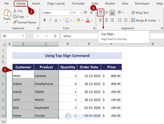
In the “Home” tab of the Excel ribbon, you will find a dedicated “Alignment” group that provides multiple options to align your cell content. You will find the “Top Align” command that aligns text to the top of the cell border. Using the “Top Align” command is the most popular and common way to top align in Excel.
To make your cell content top align using the “Top Align” command, follow these steps:
- Select the cells you want to top-align.
Here, we have selected the range B5:C10. - Go to the “Home” tab on the Excel Ribbon.
- In the “Alignment” group, select the “Top Align” icon.
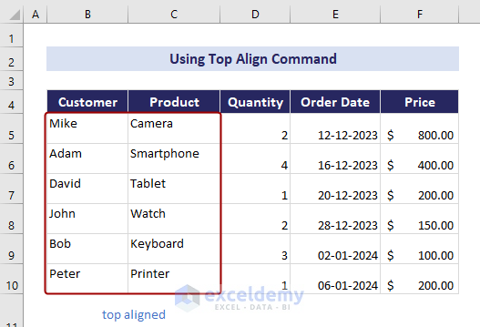
 In the image below, you can see the selected range has been top-aligned.
Note: To top-align in Excel, you can use a keyboard shortcut. Just select the desired cells and press Alt + H + A + T for instant alignment.
Using Format Cells Dialog Box
The “Format Cells” dialog box offers additional control and customization over the alignment. It provides alignment options beyond the basic top, middle, and bottom alignments. You can adjust text orientation, control text within merged cells, and much more. The dialog box provides more detailed and precise control if you need to set specific margins, indentation, or other alignment-related settings.
To top-align in Excel using the Format Cells dialog box, follow these steps:
- Select the range of cells.
- Right-click on your mouse.
- From the context menu, choose Format Cells.
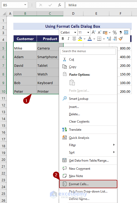 Here, the Format Cells dialog box will appear.
 - In the “Format Cells” dialog, go to the Alignment tab > Text alignment > Vertical drop-down > Top > OK.
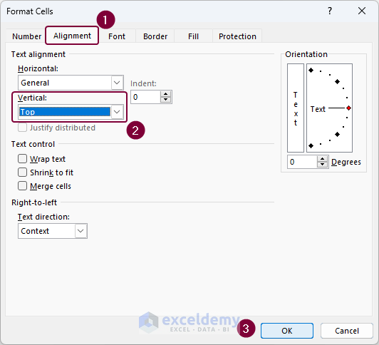 As a result, Excel will top-align your cell content. Here, we have selected the range B5:C10 to make it top-aligned.

Note: You can also launch the “Format Cells” dialog box by pressing Ctrl + 1 or clicking the Alignment Settings arrow in the Alignment group of the Home tab.
Read More: How to Change Alignment in Excel
Download Practice Workbook
Download this practice workbook for practice while you are reading this article.
Conclusion
So, you can top align in Excel using the Alignment options from the “Home” tab and the “Format Cells” dialog box. The Alignment group doesn’t need too much navigation to align text and numbers in a cell. The keyboard shortcut is also helpful for navigating quickly if you find it easy to remember. And the “Format Cells’ dialog box provides additional customization for alignment.
Frequently Asked Questions
How many types of alignments are there in Excel?
In Excel, there are two primary alignment types: horizontal and vertical. Each type has three categories. For horizontal alignment: left align, center align, and right align. And for vertical: top align, middle align, and bottom align. You will find all these alignment options in the “Alignment” group on the “Home” tab.
How do I undo an alignment in Excel?
To undo an alignment in Excel:
- Select the cell or cells with the applied alignment you wish to undo.
- Navigate to the “Home” tab and locate the “Alignment” group.
- Within the “Alignment” group, uncheck any alignment options.
- Click “OK” to apply the changes and revert the alignment.
How do I rotate text in Excel?
Rotating text in Excel is simple with these steps:
- Select the cell or range containing the text you want to rotate.
- Navigate to the “Home” tab.
- In the “Alignment” group, find the “Orientation” button.
- Click on the “Orientation” button to reveal a drop-down menu.
- Choose the desired rotation option.
- Click “OK” to apply the rotation.
Related Articles
- [Fixed!] Excel Cell Alignment Not Working
- How to Bottom Align in Excel
- How to Apply Center Horizontal Alignment in Excel
<< Go Back to Alignment | Format Cells | Learn Excel
Get FREE Advanced Excel Exercises with Solutions!
