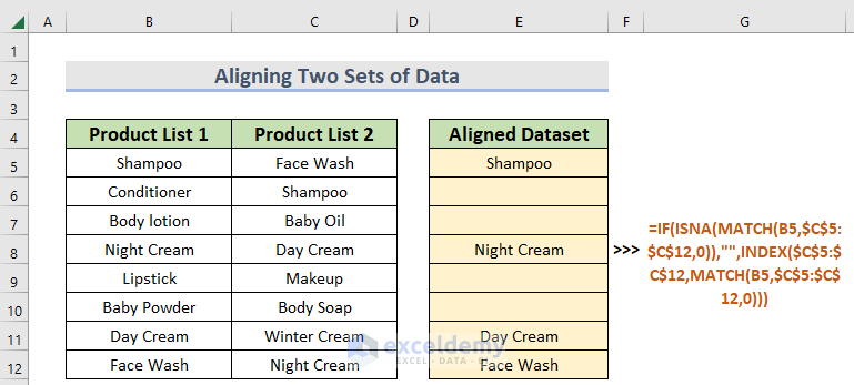
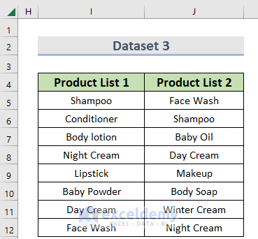
Below is a dataset showing two columns: Product List 1 and Product List 2. Next to them is a separate column, Aligned Dataset, where the aligned data will appear.
Method 1 – Using the VLOOKUP Function
Steps:
- In cell I5, enter =VLOOKUP
- Select the second dataset,
- Click cell F4 and enter a $ sign.
- Press 1,0).
- Enter the following formula:
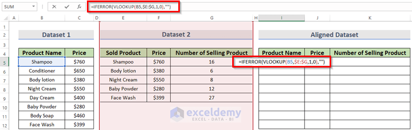
=VLOOKUP(B5,$E:$G,1,0)- If the name doesn’t match it shows Not Applicable (N/A). To avoid N/A, let’s expand the formula further.
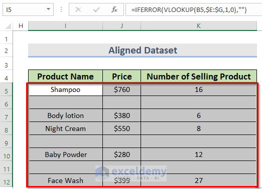
=IFERROR(VLOOKUP(B5,$E:$G,1,0),””)We have added the IFERROR function with the previous formula.
This is for the first column.
If we want to fetch the second column,
- Enter the following formula in cell J5 :
=IFERROR(VLOOKUP(B5,$E:$G,2,0),"")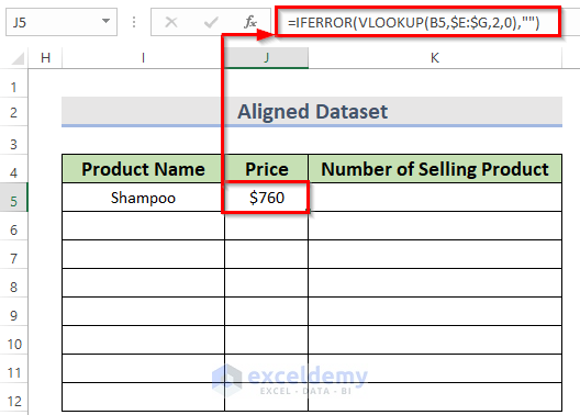
- For the third column, enter the following formula in cell K5:
=IFERROR(VLOOKUP(B5,$E:$G,3,0),"")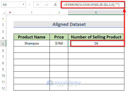
- Once we enter all the columns,
- Copy the whole formula, select the rest of the columns, and paste it.
Now, we can see that the dataset has been aligned according to column B.
Read More: All Types of Alignment in Excel (Explained in Detail)
Method 2 – Merging IF, ISNA, MATCH & INDEX Functions
In the following example, there are two sets of data. The first dataset contains some product names that are in Product List 1, and the second dataset also contains some product names that are in Product List 2. Some products are similar, so we are going to align those products.
Steps:
- Enter the following formula into the first column in the aligned dataset:
=IF(ISNA(MATCH(B5,$C$5:$C$12,0)),"",INDEX($C$5:$C$12,MATCH(B5,$C$5:$C$12,0))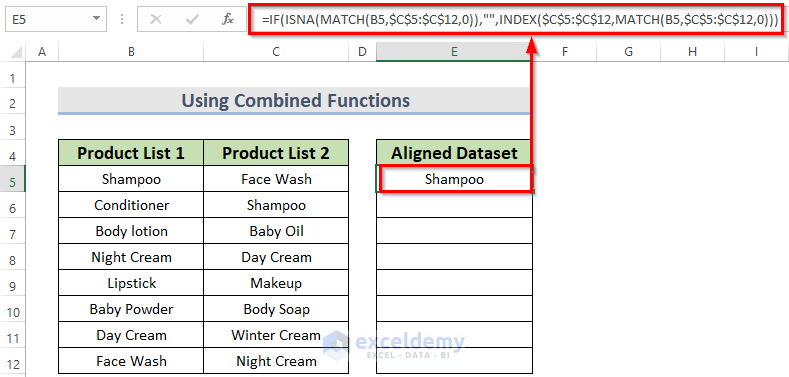
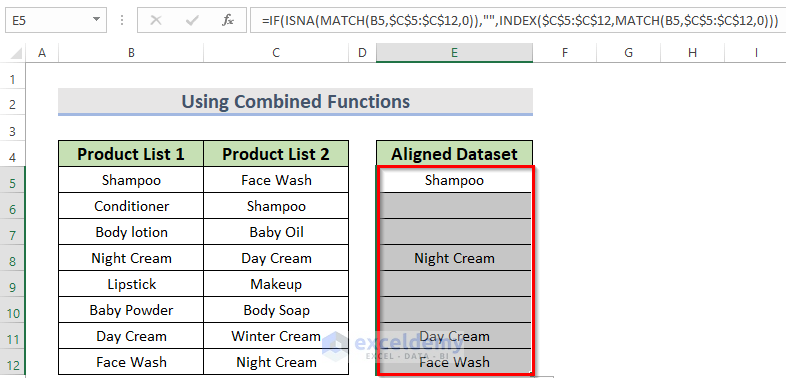
- Use the Fill Handle tool down to all the cells we want to apply this formula.
We can see all the values in the two datasets are aligned with the duplicated values.
Formula Breakdown
- MATCH(B5,$C$5:$C$12,0)—> The MATCH function will find the exact match of B5 cell value within the $C$5:$C$12 array.
- Output: 2.
- Now, INDEX($C$5:$C$12,2)—>Here the INDEX function will return the 2nd row from the given array $C$5:$C$12.
- Output: “Shampoo”.
- Similarly, MATCH(B5,$C$5:$C$12,0)—> turns 2.
- So, IF(ISNA(2),””, “Shampoo”)—> this will be the final expression of the formula. The ISNA function will examine whether the cell value is error or valid. As 2 is a valid number so ISNA function will give FALSE so the IF function will show “Shampoo” as output, on the other hand it will show a void space.
Read More: How to Align Columns in Excel (4 Easy Methods)
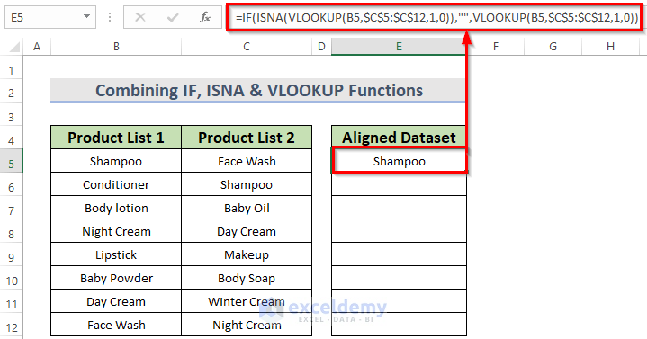
Method 3 – Combining IF, ISNA & VLOOKUP Functions
Steps:
- Enter the following formula in cell E5:
=IF(ISNA(VLOOKUP(B5,$C$5:$C$12,1,0)),"",VLOOKUP(B5,$C$5:$C$12,1,0))- Press ENTER.
Formula Breakdown
- VLOOKUP(B5,$C$5:$C$12,1,0)—> will return “Shampoo” where this VLOOKUP function is looking up for the B5 cell value, within $C$5:$C$12 this array. And 1 is the column index number.
- Then, ISNA(“Shampoo”)—> is the logical test for the IF function. Here, the ISNA function will check whether the value is an error or not. So, this will give FALSE as output.
- Then, the IF function will return a void space when the logical test is TRUE otherwise will operate VLOOKUP(B5,$C$5:$C$12,1,0) this operation.
- VLOOKUP(B5,$C$5:$C$12,1,0) this is a similar operation to the first one. Where this VLOOKUP function is looking up for the B5 cell value, within $C$5:$C$12 this array. And 1 is the column index number. 0 is for the exact match.
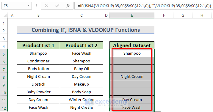
- Drag the Fill Handle icon to paste the used formula respectively to the other cells of the column.
You will get all the Aligned datasets that are duplicated in both datasets.
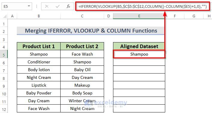
Method 4 – Merging IFERROR, VLOOKUP & COLUMN Functions
Steps:
- Enter the following formula in cell E5:
=IFERROR(VLOOKUP(B5,$C$5:$C$12,COLUMN()-COLUMN($E5)+1,0),"")- Press ENTER.
Formula Breakdown
- Here, COLUMN()-COLUMN($E5)+1 is the number of the column index for the VLOOKUP function. The COLUMN function gives the numerical representation of a given column. As the formula is used in the E column, COLUMN() becomes {5}. Also, COLUMN($E5) turns {5}. Ultimately, COLUMN()-COLUMN($E5)+1 will be 5-5+1 which is equal to 1.
- So, the formula will be as VLOOKUP(B5,$C$5:$C$12,{1},0). In this term, the VLOOKUP function will search for the value situated in the B5 cell, within the $C$5:$C$12 array. Then, 1 is the column index number and 0 denotes exact matching.
- Lastly, the IFERROR function will check whether the value is an error or not.
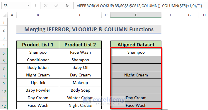
- Drag the Fill Handle icon to paste the used formula respectively to the other cells of the column.
You will get all the Aligned datasets that are duplicated in both datasets.
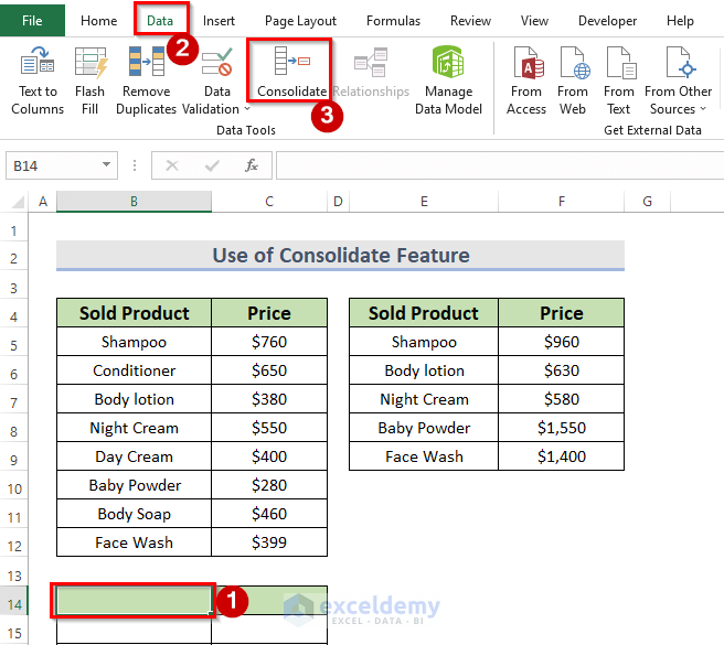
Method 5 – Using the Consolidate Feature
Steps:
You have to keep a common column header along with numerical values within those two datasets. The Consolidate feature will use them to do the calculation.
- Select cell B14.
- From the Data tab >> click on the Consolidate feature, which belongs to Data Tools.
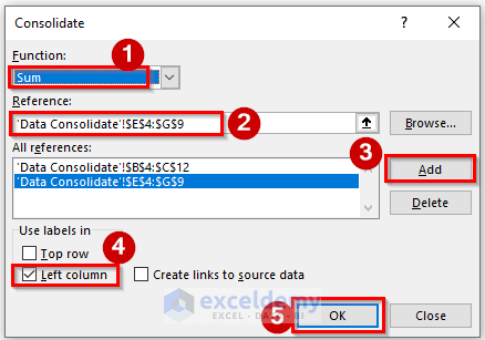
A new dialog box named Consolidate will appear.
- Choose the function. We have chosen the SUM function. So, the Consolidate feature will add the prices for the same product. Say, in the first dataset, there is Sampoo in the B5 cell, which price is $760. Now, this Consolidate feature will search for Sampoo in the second dataset. If it gets one, then it will add that price to the $760. So, here the output will be $760+$960 for the product Shampoo.
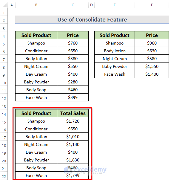
Below are the final results.
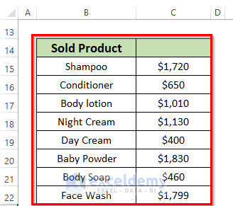
You can change the column header to a suitable one. We have changed the column header to Sold Product, and Total Sales.
Read More: How to Maintain Excel Header Alignment (with Easy Steps)
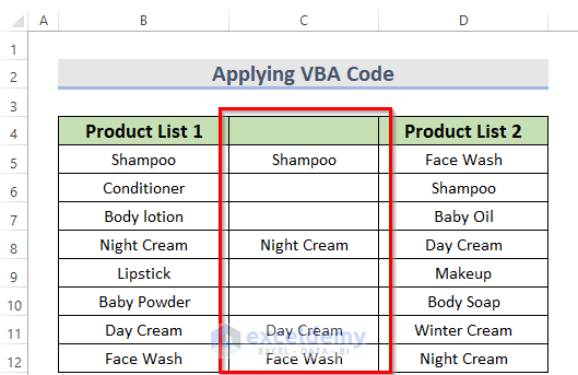
Method 6 – Employing VBA Code
Steps:
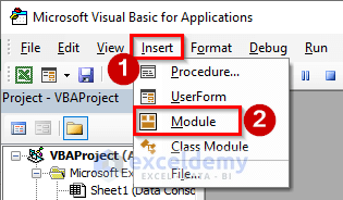
- Go to the Developer Tab and select Visual basic. This will open the visual basic editor.

- Click the Insert drop-down and select Module. This will insert a new module window.
- Or we can open the visual basic editor by right-clicking on the sheet from the sheet bar and then going to View Code.
- Enter the VBA code here:
VBA Code:
Sub Align_duplicates()
Dim my_rnge As Range
Set my_rnge = Range([B4], Cells(Rows.Count, "B").End(xlUp))
my_rnge.Offset(0, 1).Columns.Insert
With my_rnge.Offset(0, 1)
.FormulaR1C1 = _
"=IF(ISNA(MATCH(RC[-1],C[1],0)),"""",INDEX(C[1],MATCH(RC[-1],C[1],0)))"
.Value = .Value
End With
End Sub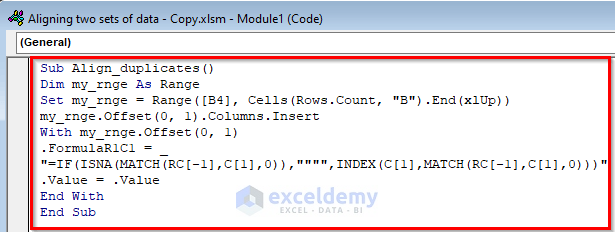
Code Breakdown
- Here, we have created a Sub Procedure named Align_duplicates.
- Next, declare a variable my_rnge as Range.
- After that, we used a formula to align the duplicate values from two sets of data.
- Now, Save the code then go back to Excel File.
- From the Developer tab >> select Macros.
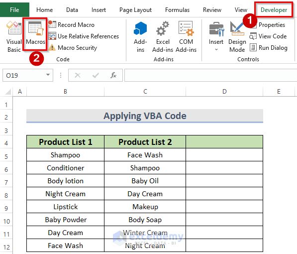
- Run the code.
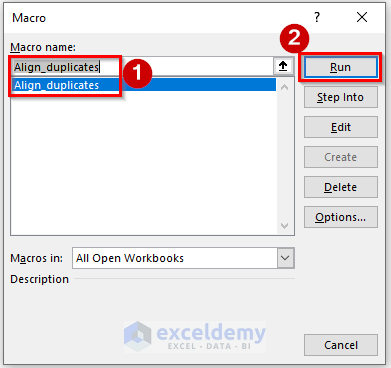
- This will insert a new column and align all the duplicate values in this new column from the two sets of data. We can see our desired result.
Read More: Excel Align Matching Values in Two Columns
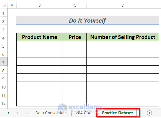
Practice Section
Now, you can practice the explained method by yourself.
Download the Practice Workbook
You can download the workbook and practice with them.
Related Articles
- How to Apply Alignment in Excel Conditional Formatting
- Excel VBA to Set Vertical Alignment (5 Suitable Examples)
- [Fixed!] Excel Cell Alignment Not Working (5 Possible Solutions)
- Align Numbers in Excel (6 Simple Methods)


On the code : =IF(ISNA(MATCH(B5,$C$5:$C$12,0)),””,INDEX($C$5:$C$12,MATCH(B5,$C$5:$C$12,0))
What if I have on column “D” a price for each product and each time I pull the item on “aligned dataset” it brings as well the price next to it ?
Hello Luis,
Thank you for sharing your problem with us. As per your referred formula, I assume it is difficult to insert each product’s price in Column D for alignment. Because you need to have 2 separate datasets comprising Products and their Prices. Only after that, you can align them individually based on each category. For this, go through the following solutions that we described in this article.
Using VLOOKUP Function to Line up Two Sets of Data in Excel
https://www.exceldemy.com/align-two-sets-of-data-in-excel/#1_Using_VLOOKUP_Function_to_Line_up_Two_Sets_of_Data_in_Excel
Use of Consolidate Feature for Summing Up Values within Two Sets of Data in Excel
https://www.exceldemy.com/align-two-sets-of-data-in-excel/#5_Use_of_Consolidate_Feature_for_Summing_Up_Values_within_Two_Sets_of_Data_in_Excel
I hope it will help you. Let us know your feedback.
Thank you.
Regards,
Sanjida Mehrun Guria
Excel VBA & Content Developer
ExcelDemy