Excel Align Matching Values in Two Columns

This article will guide you to understand how to align matching values in two columns in Excel based on the first column in the worksheet. Finding matching values in Excel worksheets is a common task we do for data analysis.

Download Practice Book

2 Methods to Align Matching Values in Two Columns in Excel

Assume two fruit shops (Shop A and Shop B), both selling varieties of seasonal fruits and we have got the product lists. We want to find out the common items they have in these product lists. We can apply formulas as well as VBA code to explore the idea. Here is the dataset; we are going to work with to show the methods:

1. Use Formula for Aligning Matching Values in Two Columns in Excel

1.1 Using IF, ISNA, INDEX & MATCH Function 

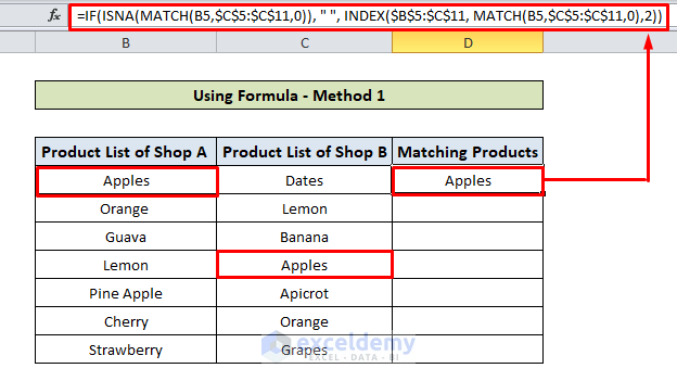
In this method, we used the IF function, the ISNA function, the INDEX function, and the MATCH function to develop a formula like this:

We are going to use this formula to align similar values from product lists of Shop A and Shop B.

• Put the above formula in the D5 cell and press Enter.

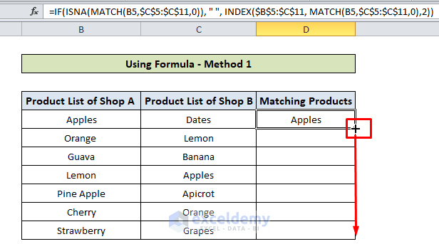
• Now, double-click on the autofill handle icon(+) on the bottom-right corner of cell D5 or drag it down through the column.

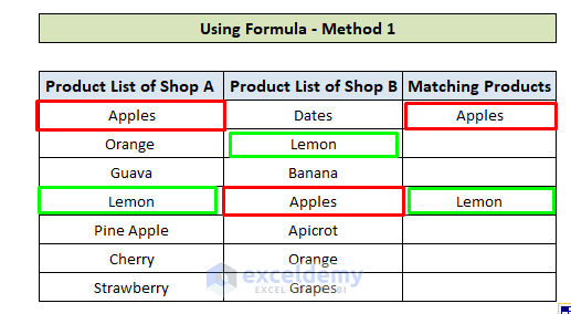
• We see the Matching Products column holds two matching items Apples and Lemon as an output.

Formula Breakdown:

• In the condition argument of the IF function:

At first, the MATCH function checks each of the items from Shop A whether it matches with the products of Shop B. If there is a match, it returns the position of the matching item in the column Shop B.

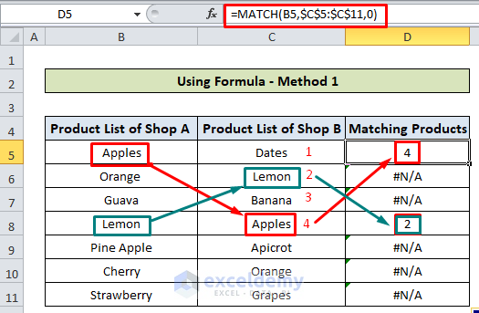
• The output of the MATCH function is then used as input of the ISNA function which returns TRUE for #N/A and FALSE for values we got from matching items.

• Now, this result is used as the condition of the IF function which returns blank for TRUE values and the name of the matching products for FALSE values.

Now, let’s break down how we get the name of the product.

We used the INDEX function to get the name of the product. Firstly, we selected both of the columns (Shop A and Shop B) as arrays, then the MATCH function gave us row_num and we put 2 as column_num.

1.2 Using IF, COUNTIF, INDEX & MATCH Function

The second formula, which is almost similar to the first one, has the COUNTIF function in the condition argument of the IF condition. Let’s follow the steps to get the matching values of two product lists of our dataset.

• In the D5 cell, lets put the formula below:

and hit ENTER.

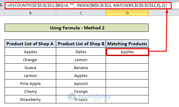
• Now, get the autofill handler and drag it through D5 to D11 to get the desired result.

Formula Breakdown:

• In the condition of  the IF function:

At first, the COUNTIF function checks each of the items from Shop A whether it matches with the products of Shop B. If there is a match, it returns the number of items in Shop B that matches with each of the items in Shop A.

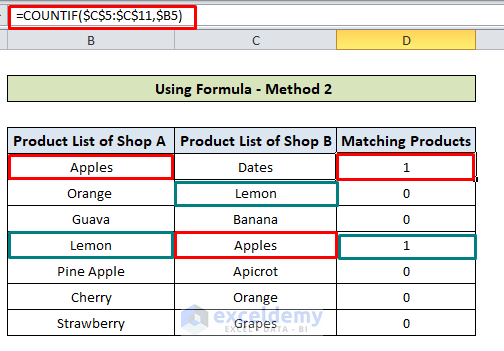
• Then we used =COUNTIF ($C$5:$C$11,$B5)=0 formula that returns FALSE for 0 values(non matching) and TRUE for otherwise(matching values).

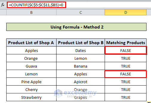
• Now, this result is used as the condition of the IF function which returns blank for TRUE values and the name of the matching products for FALSE values.

Now, let’s break down how we get the name of the product.

We used the INDEX function to get the name of the product. Firstly, we selected both of the columns (Shop A and Shop B) as arrays, then the MATCH function gave us row_num and we put 2 as column_num.

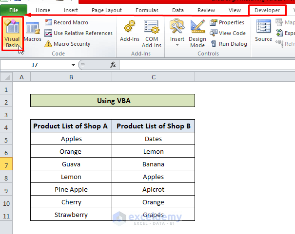
2. Line Up Matching Values Executing VBA Code in Excel

Using simple VBA code is also an easy solution to the problem of lining up the matching values in two columns in MS Excel. Let’s see how can we perform this:

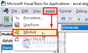
• Go to the Developer tab and click the Visual Basic option.

• It would open up the Visual Basic editor. From here, create a new Module from the Insert tab option.

• Finally, we need to put the code and run (F5) it.

Sub alignmatchingvalues() 
Dim rngA As Range
 Set rngA = Range([B1], Cells(Rows.Count, "B").End(xlUp))
 rngA.Offset(0, 1).Columns.Insert
 With rngA.Offset(0, 1)
 .FormulaR1C1 = _ 
"=IF(ISNA(MATCH(RC[-1],C[1],0)),"""",INDEX(C[1],MATCH(RC[-1],C[1],0)))" 
.Value = .Value 
End With
 End Sub

• A new column having the matching values has been inserted between the products lists columns. Let’s name it Matching Products.

Conclusion

Finally, we reach the end of the article which enlightens us to align matching values in two columns in Excel with examples. Any questions or suggestions please leave a message in the comment box.