How to Use the Excel Cell Format Formula (4 Methods)

What is Cell Formatting in Excel?

Cell formatting involves adjusting or changing the appearance of a cell without altering its original value.

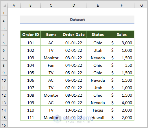
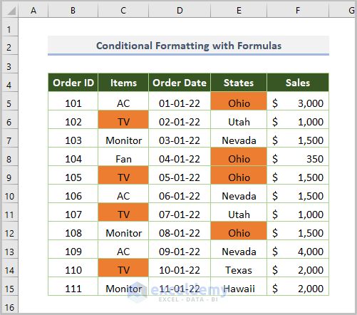
In this analysis, we’ll work with a dataset containing item names, order IDs, dates, states, and sales.

Method 1 – Cell Format Using the TEXT Function

The TEXT function converts a value to text in a specific number format. Let’s explore how to use it:

1. Syntax: =TEXT(value, format_text)
2. Example: =TEXT(B5, C5)

In the example above:

• B5 represents the cell with the value.
• C5 specifies the format text.

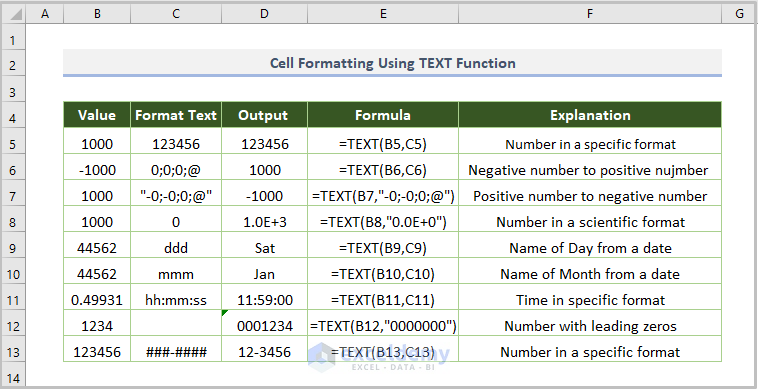
The TEXT function can:

• Convert negative values (e.g., “-1000” becomes “1000” and vice versa).
• Display values in scientific notation.
• Extract day and month names from dates.
• Add leading zeros to numbers.

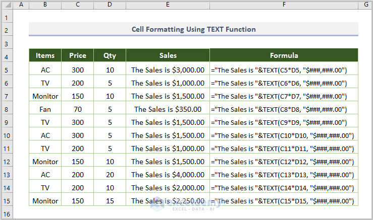
To find the sales amount (product of price and quantity) with the text “The Sales is,” use this formula:

Here, C5 is the price cell, D5 is the quantity, and $###,###.00 is the desired dollar currency format.

Method 2 – Cell Format Using Conditional Formatting

Conditional Formatting is a powerful tool in Excel that changes cell colors based on specified conditions. Let’s explore some specific applications:

2.1. Highlighting Specific Words in the Dataset

Suppose you want to highlight items like TV and states like Ohio in your dataset. Follow these steps:

• Select the cell range B5:F15.
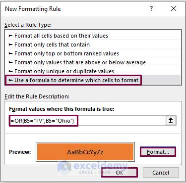
• Go to the Home tab > Conditional Formatting > New Rule.

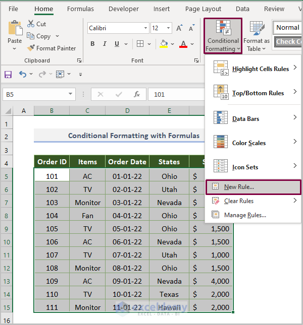
• Choose Use a formula to determine which cells to format.
• Enter this formula under Format values where this formula is true:

Here, B5 is the cell of AC.

• Specify the desired highlighting color and click OK.

The output will highlight occurrences of TV and Ohio.

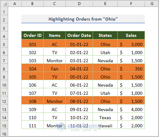
To change the color of items from Ohio states, use this formula:

Here, E5 is the starting cell of the states field.

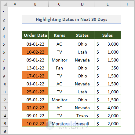
2.2. Highlighting Dates in Next 30 Days

To identify and highlight dates within the next 30 days, use this formula in the New Formatting Rule dialog box:

Here, B5 represents the order date. The formula combines the AND and NOW functions.

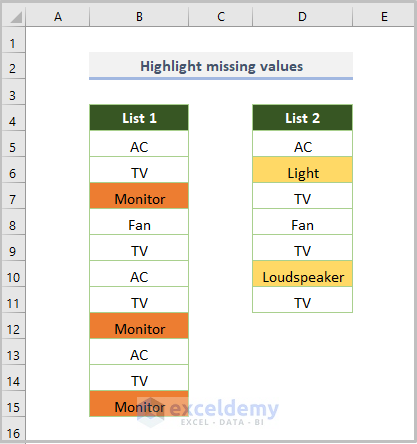
2.3. Highlighting Missing Values 

You can show missing values by synchronizing lists using conditional formatting. Use these formulas:

Here, D5:D11 is the cell range of List 2, and B5 is the starting cell of List 1.

And the formula for list 2 is-

Here, B5:B15 is the cell range of List 1 and D5 is the starting cell of List 2.

2.4. Applying Multiple Criteria as Cell Format

We can use AND logic with multiple criteria across the entire dataset and highlight the output using conditional formatting.

For instance, let’s highlight items with a price less than or equal to $300 and sales greater than or equal to $2000.

For this, put the following formula in the New Formatting Rule dialog box:

Here, E5 represents the starting cell for prices, and G5represents the starting cell for sales.

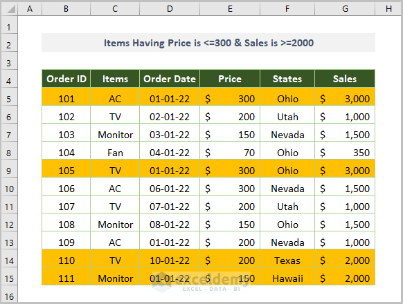
As a result, only 4 items meet the criteria of having a price less than or equal to $300 and sales greater than or equal to $2000.

Method 3 – Cell Format Formula Using VBA Coding

Let’s explore how to apply the VBA Format function to convert values into specific formats:

Step 1: 

Open a module by clicking Developer>Visual Basic>Insert>Module.

Step 2: 

Copy the following code into your module:

Sub Format_func()
Range("C5").Value = Format(Range("B5"), "Currency")
Range("C6").Value = Format(Range("B6"), "Long Date")
Range("C7").Value = Format(Range("B7"), "True/False")
Range("C8").Value = Format(Range("B8"), "Standard")
Range("C9").Value = Format(Range("B9"), "Fixed")
Range("C10").Value = Format(Range("B10"), "Long Time")
Range("C11").Value = Format(Range("B11"), "Short Time")
End Sub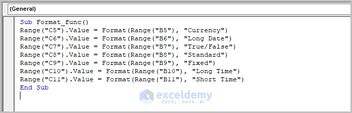

Step 3:

Run the code.

Notes:

The following things are essential in the above VBA code.

• Worksheet name: The worksheet name in this example is “Format_func”.
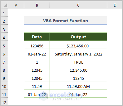
• Logic: The Format  function returns values in specific formats.
• Input Cell: We use cells B5, B6, etc., as input.
• Output range: The output ranges are C5, C6, etc.

After running the code, the output will be as follows.

Method 4 – Cell Format Utilizing LEFT, MID, RIGHT, LEN & FIND Function

Let’s explore some applications of the LEFT, RIGHT, MID, FIND, and LEN functions:

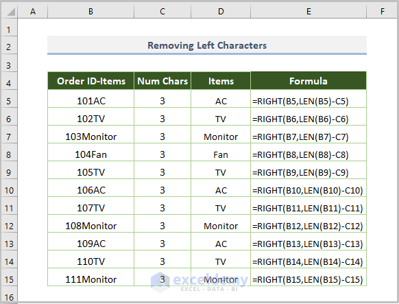
RIGHT Function:

• Removes characters from the left side of the Order ID-Items string.

Formula:

• • Here, B5 is the cell containing the combined Order ID-Items, and C5 represents the number of characters to remove.

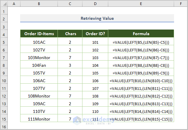
Formatting Cells in Numeric Format:

• Converts a combination of text and numbers (Order ID-Items) into numeric format.

Formula:

• • B5 is the cell containing the combined Order ID-Items, and C5 is the starting cell for Chars.

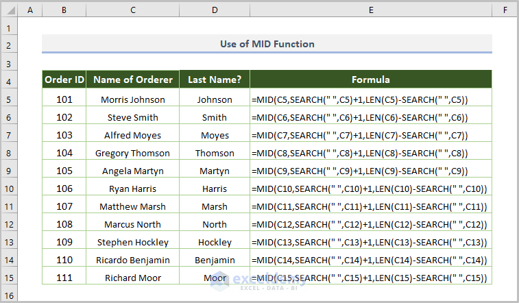
MID Function:

• Extracts the last name from the Name of Orderer.

Formula:

• • Here, C5 is the starting cell of Name of Orderer.

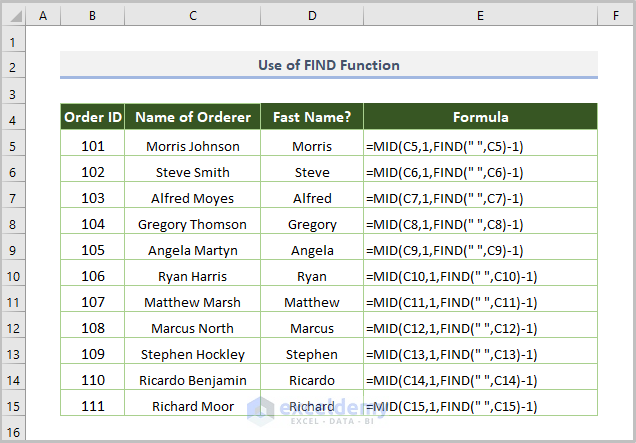
FIND Function:

• Retrieves the first name from the Name of Orderer.

Formula:

• • Here, C5 is the starting cell of Name of Orderer.

These unconventional methods can be helpful for extracting and organizing data in specific cell formats.

Download Practice Workbook

You can download the practice workbook from here:

Related Article

• [Solved] Excel Formatting Not Working Unless Double Click Cell

<< Go Back to Excel Cell Format | Learn Excel