In this article, you will get five tips on how to pass an Excel assessment test. Additionally, there will be some exercises for your practice. You will need an advanced understanding of Excel to solve all the problems. Moreover, you should know the following: INDEX, MATCH, SUMIF, LEFT, SEARCH, MID, RIGHT, FIND, SUBSTITUTE, LEN, COUNTIF, COUNTBLANK, and VLOOKUP functions; the Fill Handle, ways to AutoFill the formulas, custom cell formatting, conditional formatting, working with the chart elements, inserting a pie chart, Flash Fill, Filter feature, the Sort feature and adjustment of background cell color features to find the solutions to the problems. You should use the Excel 2010 version of Excel to solve all the problems without any issues.
Problem Overview
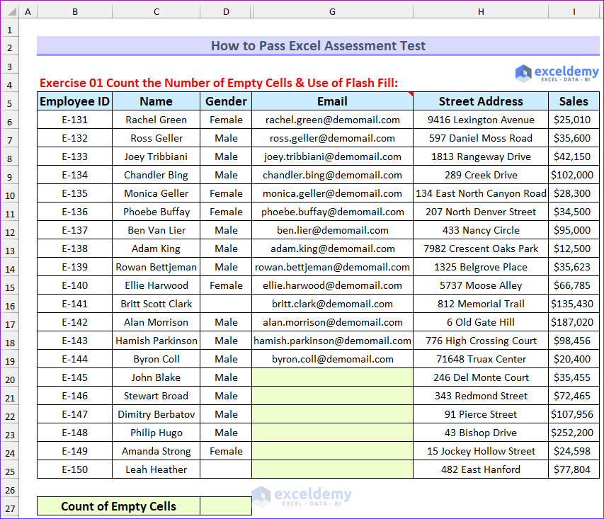
In this section, we will list five tips to pass an Excel assessment test. After that, we will provide some Excel exercises for your practice. The “Problem” sheet shows the exercises and the “Solution” sheet shows the problems worked out. The following image shows the first problem of this article. We’ve hidden some columns for better visualization.
Five Tips to Pass an Excel Assessment Test
- Firstly, ask about the Excel version. Some features are not available in earlier versions of Excel. Moreover, newer formulas are shorter and simpler. Therefore, if you are used to modern formulas and don’t know how to perform the same task with older formulas, you will be in trouble. So, if it is possible then ask about the Excel version or know alternative ways to solve a problem. Our site provides alternative solutions in most of the articles, so it is a great place to learn.
- Secondly, learn keyboard shortcuts to save time. The tests are time constrained, so learning keyboard shortcuts will save you a ton of time. For example, if you want to work with VBA then you will need to enable the developer tab and click on Visual Basic from that. Alternatively, you can press Alt+F11 to do so. It saves a ton of time.
- Thirdly, go through your job description. This will steer you to the right direction about taking preparation for the test. If you apply for a data entry job, then learn about data validation. If you apply for a data analyst position, then learn the pivot table, use of insert chart and conditional formatting features. Lastly, most of the test will include some lookup functions (VLOOKUP, INDEX-MATCH, HLOOKUP, etc.), learn these.
- Fourthly, be confident. You should be calm and confident when taking the test. If you get nervous, then practice breathing exercises to reduce the stress.
- Fifthly, practice more. We have thousands of articles related to Excel. So, this site is an Excellent source of learning topics and practicing exercises.
Practice Exercises
Now, we will list some problems. There are eight exercises for your practice.
- Exercise 01 Count the Number of Empty Cells & Use of Flash Fill: There are two tasks in this exercise. Firstly, find the number of the blank cells inside the dataset. Finally, fill the email rows (with the format “[email protected]”).
- Hint: You can fill in the rows in various ways. The easiest way to do so is to use the Flash Fill feature.
- Exercise 02 Lookup Values Using VLOOKUP and INDEX MATCH: Six employee IDs are given. Your task is to find the name and position of the employee. Firstly, using the VLOOKUP function and then using the INDEX MATCH functions.
- Hint: An invalid employee ID is given. You need to use the IFERROR or IFNA function to resolve the issue.
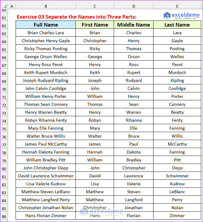
- Exercise 03 Separate the Names into Three Parts: The full name of twenty four people is provided, your task is to use three formulas to separate the names into first name, middle name, and last name.
The following animated image shows the formula to return the first name of the employee.

- Exercise 04 Find Sales Statistics Using Formulas: Use different formulas to find the number of female employees, sales generated by them, employees joined before May 2022 and the sales generated by the traveling salesperson.
- Exercise 05 Use of Filter Feature: Apply the Filter feature to show the sales values greater than $100,000. Additionally, use the Sort feature to sort the sales values by largest to smallest.
- Hint: It is better to convert the range into a table before doing the filter operation.
- Exercise 06 Create a Pivot Table: Sales values generated by five employees are given for a particular period. Apply the PivotTable feature to find the sales value originated by the employees.
- Exercise 07 Application of Conditional Formatting: Twenty employees enrolled for a course that took place for three days in the company auditorium. It was mandatory to attend the session for at least one day. Your task is to find who did not attend the course and use conditional formatting.
- Red color for 3 days absent
- Yellow color for 2 days absent
- Green color for perfect attendance (0 day absent)
- Moreover, count the number of employees present and absent for each day
- Then, apply conditional formatting (color Red) for more than six employees absent
- Exercise 08 Use of Excel Charts: In the final exercise, your task is to create two charts. Firstly, you will create a pie chart from the given data. Then, add Title, Data Labels (Percentage), and Legend to it.
- Secondly, create a combo chart from another dataset. The sales values will be on the secondary axis. Then, add the axis title, chart title, and data label to the chart.
The following image shows the solution to the third problem.
Read More: Excel Practice Test for Employment
Download Practice Workbook
You can download the Excel file from the following link.
Conclusion
Thank you for reading this article. By completing this article, we hope that you have gained knowledge about how to pass an Excel assessment test. If you have any questions or suggestions, feel free to comment below. However, remember that our website implements comment moderation. Therefore, your comment may not be instantly visible. So, have a little bit of patience, and we will solve your query as soon as possible. Keep excelling!
Get FREE Advanced Excel Exercises with Solutions!
