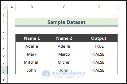
We will use the sample dataset below to demonstrate how to compare two cells in Excel.
Method 1 – Compare Two Cells Side by Side Using Equal to Sign
Steps:
- Add the following formula in Cell D5 (to compare B5 & C5).
=B5=C5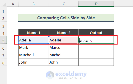
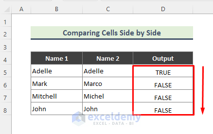
- Drag down the Fill Handle (+) to copy the formula to the rest of the cells.
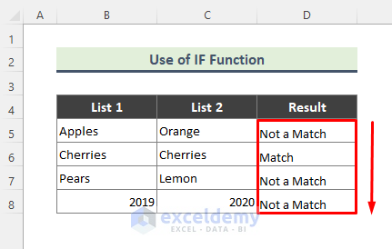
Method 2 – Use IF Function to Compare Two Cells
Steps:
- Insert the IF function in Cell D5 and select the arguments.
=IF(B6=C6,"Match","Not a Match")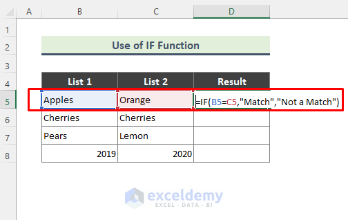
- Drag down the Fill Handle (+) of Cell D5 to copy the formula to the rest of the cells.
Method 3 – Insert Excel EXACT Function to Compare Two Cells
Steps:
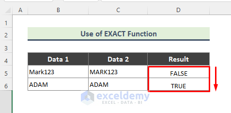
- To compare Cell B5 and Cell C5, enter EXACT function and select required cells for arguments.
=EXACT(B5,C5)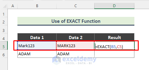
- Drag down the Fill Handle (+) of Cell D5 to copy the formula to the rest of the column.
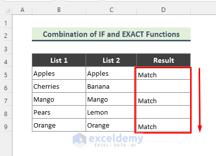
Method 4 – Combine IF and EXACT Functions to Compare Two Cells in Excel
Steps:
- To compare Cell B5 and Cell C5, enter the formula combining both functions:
=IF(EXACT(B5,C5), "Match","")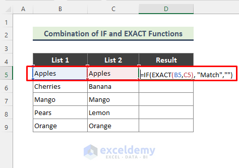
- You will get the following result.
Read More: Check If Multiple Cells Are Equal in Excel
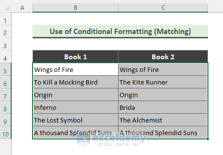
Method 5 – Highlight Matching Data to Compare Two Cells
Steps:
- Select the dataset.
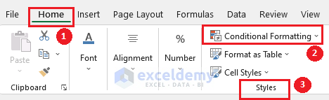
- Go to Home > Conditional Formatting from the Styles group.
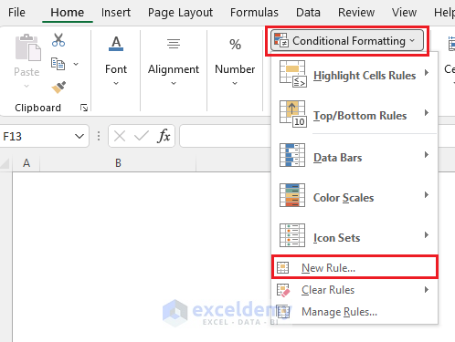
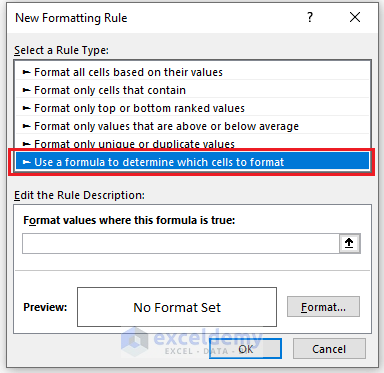
- Click New Rule From Conditional Formatting.
- A new dialogue box will show up. Select the rule “Use a formula to determine which cells to format”.
- Add the following formula in the description box.
=$B5=$C5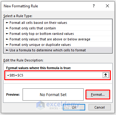
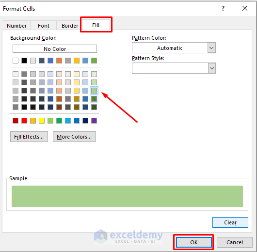
- Click the Format button, go to the Fill tab, and choose the color. Click OK.
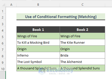
All matched cells in the two columns will be highlighted. Conversely, differently named rows would not be highlighted.
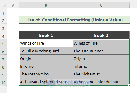
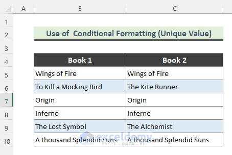
Method 6 – Compare and Highlight Two Cells with Unique Data in Excel
Steps:
- Select the dataset.
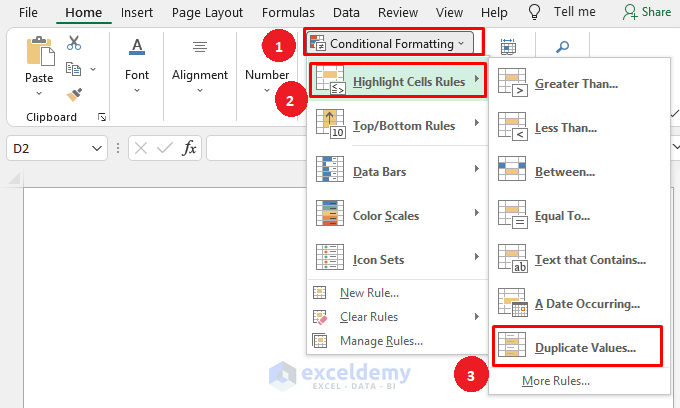
- Go to Home > Conditional Formatting from the Styles group.

- Press the Duplicate Values option from Highlight Cell Rules.
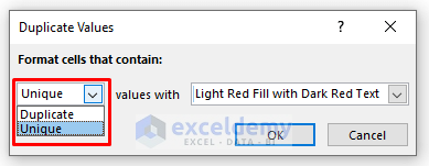
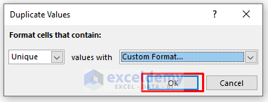
- The Duplicate Values dialogue box will show up. Choose the Unique option from the drop-down.
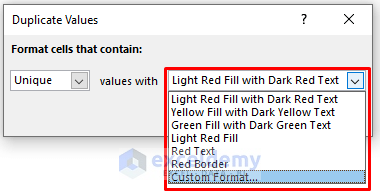
- You can also choose the color of the highlight from the drop-down by using the Custom Format option.
- Enter OK.
- All the unique values between cells are highlighted.
Read More: Compare Text in Excel and Highlight Differences
7. Use LEFT & RIGHT Functions to Compare Two Cells Partially
7.1. Compare Using LEFT Function
Steps:
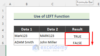
- To match the first 3 characters of Cell B5 and Cell C5, add formula using LEFT Function:
=LEFT(B5,3)=LEFT(C5,3)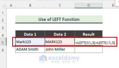
- Click Fill Handle (+) of Cell D5 to copy the formula to the rest of the column.
7.2. Compare Using RIGHT Function
Steps:
- To match the last 3 characters of cell H5 and cell I5, Insert the RIGHT function and select or type arguments. Here is the Formula:
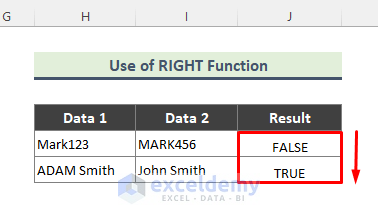
=RIGHT(H5,3)=RIGHT(I5,3)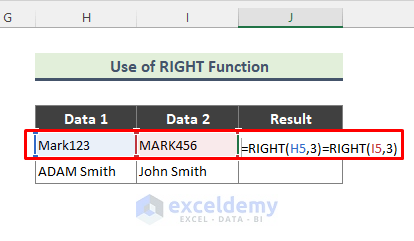
- Click the Fill Handle (+) of cell D5 to copy the formula to the rest of the column.
Method 8 – Using VLOOKUP and Find Matches in Excel
Steps:
- To match the value of Cell C5 in Column Name 1, use the formula:
=IFERROR(VLOOKUP(C5,$B$5:$B$11,1,0),"No Match")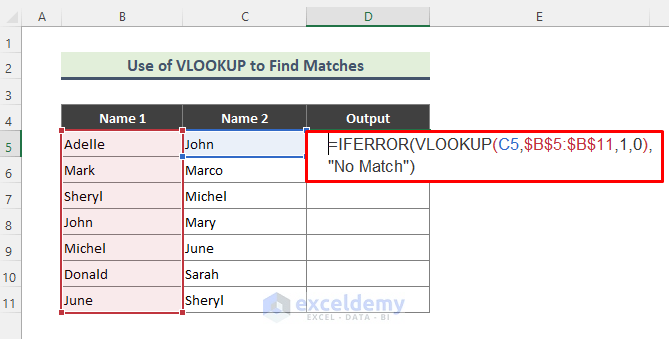
Breakdown of the Formula:
- VLOOKUP(C5,$B$5:$B$11,1,0)
The VLOOKUP function looks for a value in the leftmost column of a table and then returns a value in the same row from a column you specify. The function will look for C5 in the range B5:B11 and return:
{John}
When the function finds C6 in range B5:B11, it will return a #N/A error because C6 is not present in the prescribed range.
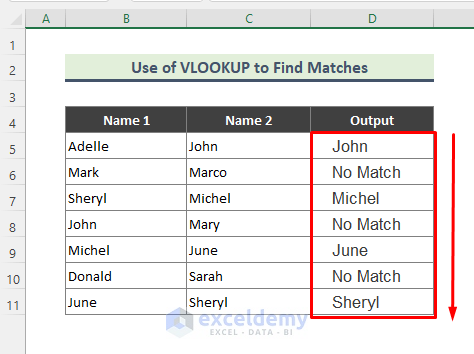
- IFERROR(VLOOKUP(C5,$B$5:$B$11,1,0), “No Match”)
The IFERROR function returns value_if_error if the expression is an error and the value of the expression itself otherwise. In our example, we have put “No Match” as an argument. As a result, when we look for C6 in the above-mentioned range, the formula returns:
{No Match}
- After entering the formula, you will get the matched name in a 3rd column. Use the Fill Handle (+) to copy the formula for the rest of the cells.
Method 9 – Using VLOOKUP and Find Differences
Steps:
- To find data in Cell C5 in Column Name 1, the formula will be:
=IF(ISERROR(VLOOKUP(C5,$B$5:$B$11,1,0)),"Not Available","Available")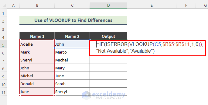
Breakdown of the Formula:
- VLOOKUP(C5,$B$5:$B$11,1,0)
The VLOOKUP function looks for a value in the leftmost column of a table and then returns a value in the same row from a column you specify. The function will return:
{John}
This is not the end result we want from this method. We want to know whether any value is present in a range or not. The next part of the formula is:
- ISERROR(VLOOKUP(C5,$B$5:$B$11,1,0))
The ISERROR function checks whether a value is an error, and returns TRUE or FALSE. So, for D5, the function will find the value of C5 in the range B5:B11 and return:
{FALSE}
The reason is, C5 is present in the mentioned range. For other cells when an error is found, it will return “TRUE”.
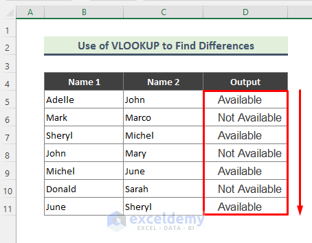
- IF(ISERROR(VLOOKUP(C5,$B$5:$B$11,1,0)),”Not Available”,”Available”)
The IF function checks whether a condition is met, and returns one value if true, and another value if false. We put “Not Available” and “Available” as arguments. For D5, the function returns:
{Available}
Step 2:
- After entering the formula you will find the differences in the Output Column.
- Use the Fill Handle (+) to copy the formula for the rest of the cells.
Read More: Return YES If 2 Cells Match in Excel
Method 10 – Compare Two Cells with Greater Than or Less Than Criteria
Steps:
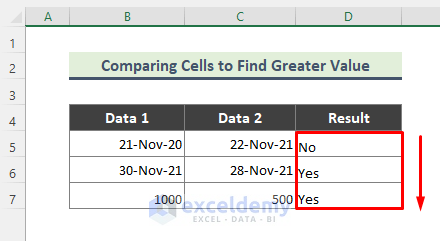
- To compare Cell B5 and Cell C5, we have used the following formula:
=IF(B5>C5,"Yes","No")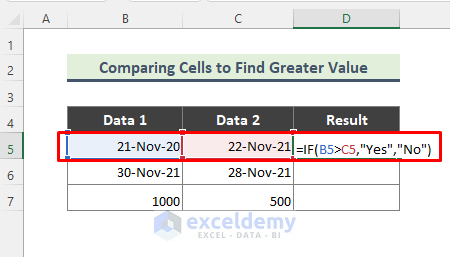
- In our dataset, the date in Cell B5 is not greater than the date in Cell C5 so the output is No.
Download Excel Workbook
Excel Compare Cells: Knowledge Hub
<< Go Back To Compare in Excel | Learn Excel
Get FREE Advanced Excel Exercises with Solutions!

In “10. Compare Two Cells with Greater Than or Less Than Criteria”, I would like to determine the actual numerical difference between the two cells and the percentage of that difference to one of the cells. Eg., if one cell is 2 and the other cell is 10 … the difference is 8, which is 80% less than 10 (10 would be the mean of my interested dataset). How to I go about writing the formula?
Thank you.
J
Hi J,
Hope you are doing well.
You can get the actual numerical difference between two cells by using subtraction (-) in the formula. In case of, percentage value use the formula given below.
=IF(AND(0<D5,D5<$D$10),(D5/$D$10)*100&"% Less Than 10",(-D5/$D$10)*100&"% Greater Than 10")If the condition is True then the formula will return the result as follows.
On the other hand, if the condition is False then the formula will return the result as follows.
Here, the AND function will return True if both the conditions are true else it will return False.
Thanks.
Regards,
Arin Islam
Amazing!!!
Hello Syed,
Thanks for your feedback and appreciation. Glad to hear that you liked our tutorial.
Keep exploring Excel with ExcelDemy!
Regards,
ExcelDemy