How to Compare Two Strings for Similarity In Excel

In this tutorial, I am going to show you 6 easy methods on how to compare two strings for similarity in excel. You can use these methods even in large datasets to find out cells that have exactly or partially similar strings. Throughout this tutorial, you will also learn some important excel tools and techniques which will be very useful in any excel related task.

Download Practice Workbook

You can download the practice workbook from here.

6 Easy Methods to Compare Two Strings for Similarity in Excel

We have taken a concise dataset to explain the steps clearly. The dataset has approximately 7 rows and 2 columns. Initially, we are keeping all the cells in General format. For all the datasets, we have 2 unique columns which are Sales Person Full Name and First Name. Although we may vary the number of columns later on if that is needed.

1. Using Highlight Cells Rules Feature

In this first method, we will see how to compare two strings for similarity using the Highlight Cells Rules in excel. Follow the steps below.

Steps:

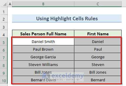
• First, select all the cells from B5 to C10.

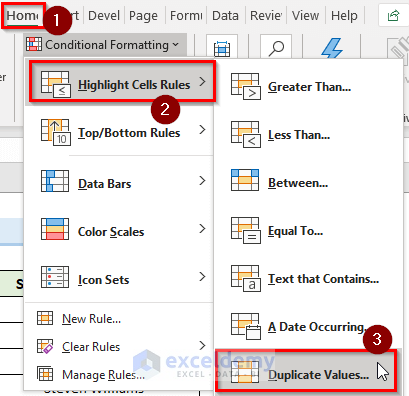
• Next, go to the Home tab and click on Conditional Formatting.
• Here, go to Highlight Cells Rules and click on Duplicate Values.

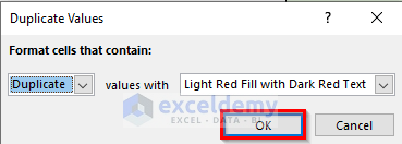
• Now, simply click on OK.

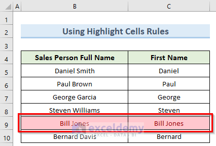
• As a result, this should highlight the values that are similar.

Read More: How to Compare Text in Excel and Highlight Differences (8 Quick Ways)

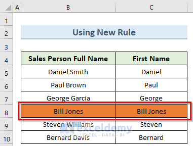
2. Applying New Rule Feature

We can also use the New Rule feature in excel which gives us custom options to compare two strings for similarity. Let us see how to do that.

Steps:

• To begin with, again select the cells from B5 to C10.

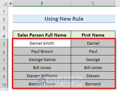
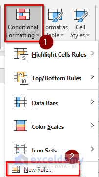
• Now, navigate to Conditional Formatting under the Home tab and click on New Rule.

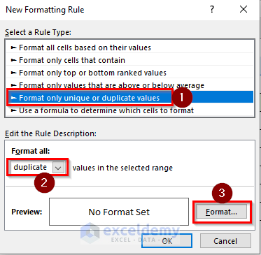
• Next, in the new window, select Format only unique or duplicate values and click on Format.

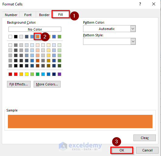
• Then, select a color under the Fill tab and click OK in this window and also in the next window.

• Consequently, this will highlight the values that are similar in the dataset.

Read More: Compare Two Cells in Excel and Return TRUE or FALSE (5 Quick Ways)

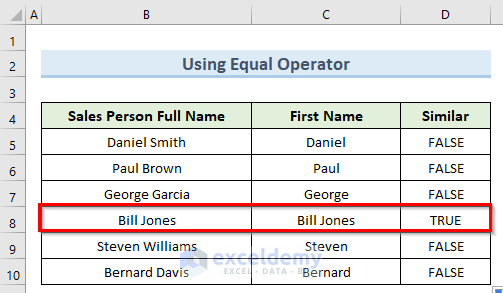
3. Utilizing Equal Operator

The equal operator in excel can evaluate whether a statement is TRUE or FALSE. We will use this symbol to quickly compare two strings for similarity. Below are the detailed steps.

Steps:

• First, go to cell D5 and insert the following formula:

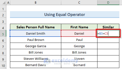
• Now, press Enter and copy this formula to the other cells using Fill Handle.
• Finally, this will give TRUE or FALSE values based on whether the values match or not.

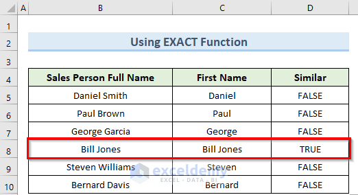
4. Comparing Using EXACT Function

The EXACT function in excel is very useful if we want to compare two text strings for similarity. For this, we just need to give the two strings as inputs to this function. Let us see the step-by-step process.

Steps:

• To begin this method, double-click on cell D5 and insert the formula below:

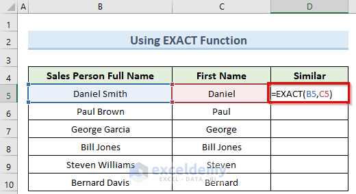
• Next, press the Enter key and consequently, this will insert TRUE if the values are exactly similar.

5. Using SEARCH Function

The SEARCH function in excel can find the position of one string inside another string. So, we should be able to use this function to compare two strings for similarity. Follow the steps below to do this.

Steps:

• To start this method, navigate to cell D5 and type in the following formula:

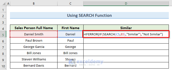
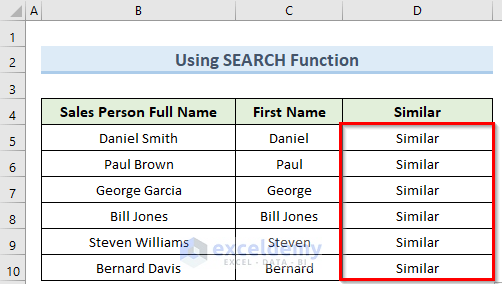
• After that, press the Enter key or click on any blank cell.
• Immediately, this will give you the result as similar or not for all the data.

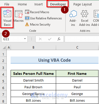
6. Applying VBA Code

If you are familiar with VBA in excel, you can easily compare two strings for similarity. Although we will write a little lengthy code, you can just copy this code into your own file. Let us see how to write VBA code for this.

Steps:

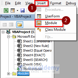
• For this method, go to the Developer tab and select Visual Basic.

• Now, select Insert in the VBA window and click on Module.

• Next, type in the formula below in the new window:

Sub Highlight()
    Dim xRg1 As Range
    Dim xRg2 As Range
    Dim xTxt As String
    Dim xCell1 As Range
    Dim xCell2 As Range
    Dim I As Long
    Dim J As Integer
    Dim xLen As Integer
    Dim xDiffs As Boolean
    On Error Resume Next
    If ActiveWindow.RangeSelection.Count > 1 Then
      xTxt = ActiveWindow.RangeSelection.AddressLocal
    Else
      xTxt = ActiveSheet.UsedRange.AddressLocal
    End If
lOne:
    Set xRg1 = Application.InputBox("Range A:", "Select Range", xTxt, , , , , 8)
    If xRg1 Is Nothing Then Exit Sub
    If xRg1.Columns.Count > 1 Or xRg1.Areas.Count > 1 Then
        MsgBox "Multiple ranges or columns have been selected ", vbInformation, "Similar or Not"
        GoTo lOne
    End If
lTwo:
    Set xRg2 = Application.InputBox("Range B:", "Select Range", "", , , , , 8)
    If xRg2 Is Nothing Then Exit Sub
    If xRg2.Columns.Count > 1 Or xRg2.Areas.Count > 1 Then
        MsgBox "Multiple ranges or columns have been selected ", vbInformation, "Similar or Not"
        GoTo lTwo
    End If
    If xRg1.CountLarge <> xRg2.CountLarge Then
       MsgBox "Two selected ranges must have the same numbers of cells ", vbInformation, "Similar or Not"
       GoTo lTwo
    End If
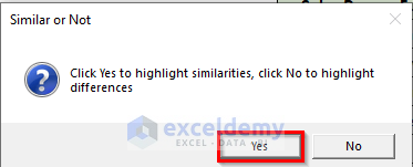
    xDiffs = (MsgBox("Click Yes to highlight similarities, click No to highlight differences ", vbYesNo + vbQuestion, "Similar or Not") = vbNo)
    Application.ScreenUpdating = False
    xRg2.Font.ColorIndex = xlAutomatic
    For I = 1 To xRg1.Count
        Set xCell1 = xRg1.Cells(I)
        Set xCell2 = xRg2.Cells(I)
        If xCell1.Value2 = xCell2.Value2 Then
            If Not xDiffs Then xCell2.Font.Color = vbRed
        Else
            xLen = Len(xCell1.Value2)
            For J = 1 To xLen
                If Not xCell1.Characters(J, 1).Text = xCell2.Characters(J, 1).Text Then Exit For
            Next J
            If Not xDiffs Then
                If J <= Len(xCell2.Value2) And J > 1 Then
                    xCell2.Characters(1, J - 1).Font.Color = vbRed
                End If
            Else
                If J <= Len(xCell2.Value2) Then
                    xCell2.Characters(J, Len(xCell2.Value2) - J + 1).Font.Color = vbRed
                End If
            End If
        End If
    Next
    Application.ScreenUpdating = True
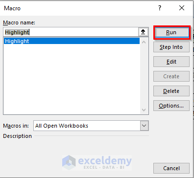
End Sub

• Then, open the macro from the Developer tab by clicking on Macros.

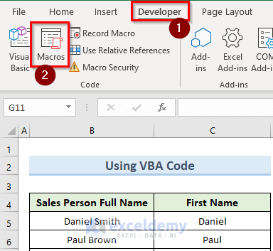
• Now, in the Macro window, select the Highlight macro and click Run.

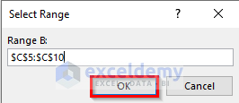
• After that, insert the first range in the Select Range window and click OK.

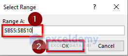
• Next, select the second range and again click OK.

• Here, press Yes to confirm.

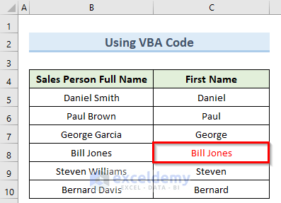
• As a result, the VBA code will highlight a similar value in cell C8.

Conclusion

I hope that you were able to apply the methods that I showed in this tutorial on how to compare two strings for similarity in excel. As you can see, there are quite a few ways to achieve this. So wisely choose the method that suits your situation best. If you get stuck in any of the steps, I recommend going through them a few times to clear up any confusion. Lastly, to learn more excel techniques, follow our ExcelDemy website. If you have any queries, please let me know in the comments.

Further Readings

• Return YES If 2 Cells Match in Excel (10 Methods)
• Compare Two Cells Using Conditional Formatting in Excel (3 Methods)
• How to Compare Two Cells and Change Color in Excel (2 Ways)
• Excel Formula to Compare Two Cells in Different Sheets (3 Examples)
• Statistical Comparison of Two Data Sets Excel
• How to Compare Addresses in Excel (11 Easy Methods)
• Compare Two Cells in Excel (10 Easy Methods)