How to Compare Text and Highlight Differences in Excel (8 Quick Ways)

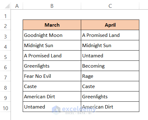
To demonstrate our Methods, we’ll use the following dataset containing the names of the best-selling books in an online shop over two consecutive months. We’ll compare them and highlight differences using some easy techniques.

Method 1 – Using the EXACT Function

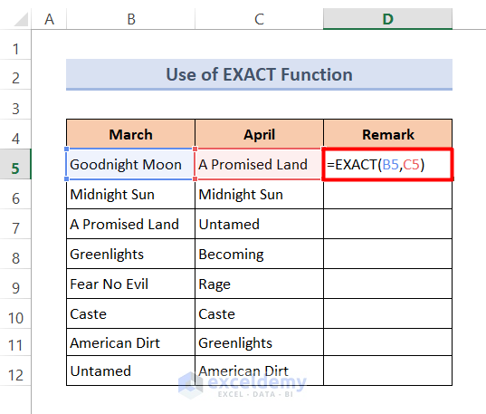
The EXACT function is used to compare two strings or data and return whether both data are an exact match or not.

To showcase the method, a new column named ‘Remark’ is added to our dataset.

Steps:

⏩Activate Cell D5.

⏩Enter the following formula:

⏩Press Enter.

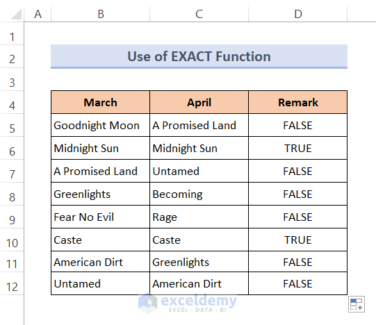
⏩Double click the Fill Handle icon to fill the formula down to D12.

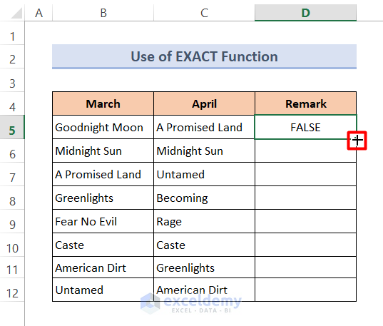
The output displays FALSE where the contents of the adjacent cells are not an exact match and TRUE when they are.

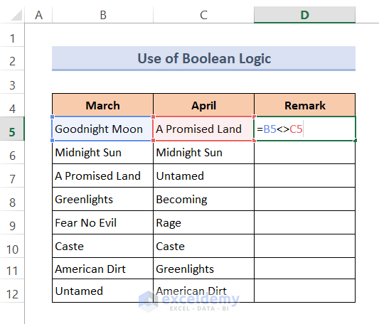
Method 2 – Using Boolean Logic

The same operation  –  returning TRUE or FALSE for an exact match in the same row – can be accomplished using simple Boolean logic.

Steps:

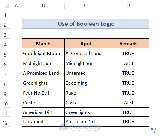
⏩Enter the following formula in Cell D5:

⏩Press Enter and double-click the Fill Handle icon to copy the formula.

Because our function returns TRUE for matches that are not an exact match, the values returned are the opposite of Method 1.

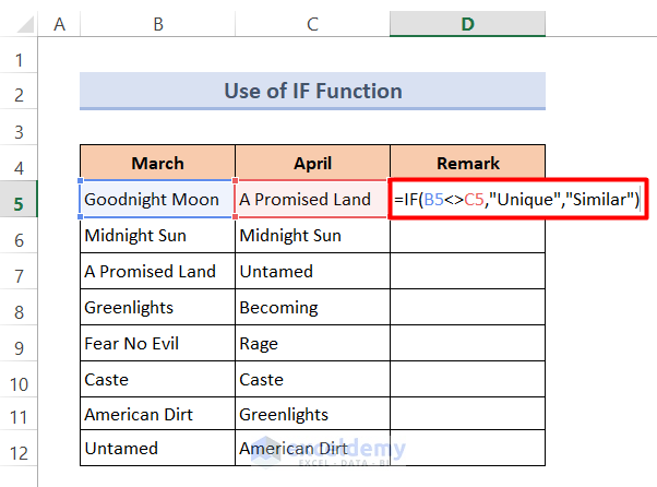
Method 3 – Using the IF Function

Combining the IF function with Boolean logic accomplishes the same result, but with customized output text. Our formula displays ‘Unique’ if the contents of cell C5 are different to cell B5, and ‘Similar’ if they are an exact match.

Steps:

⏩In Cell D5 enter the formula:

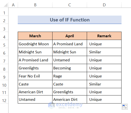
⏩Press Enter and use the Fill Handle tool to fill the other cells.

The output is the same as Method 2, but with our customized responses.

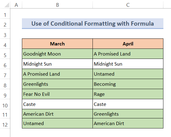
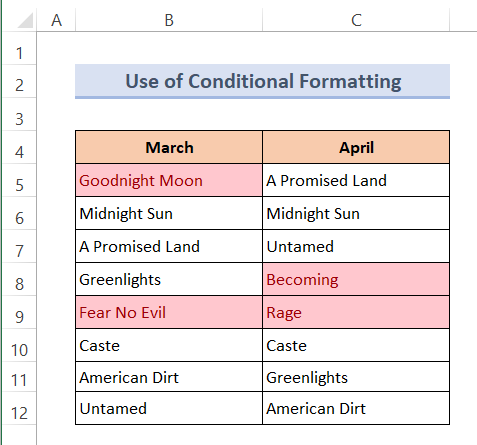
Method 4 – Using Conditional Formatting with Formula

Conditional Formatting is a very convenient method of comparing text and highlighting differences in Excel. Here we use pre-selected colors to highlight differences.

Steps:

⏩Select the data range B5:C12.

⏩Click Home > Conditional Formatting > New Rule. A formatting dialog box opens.

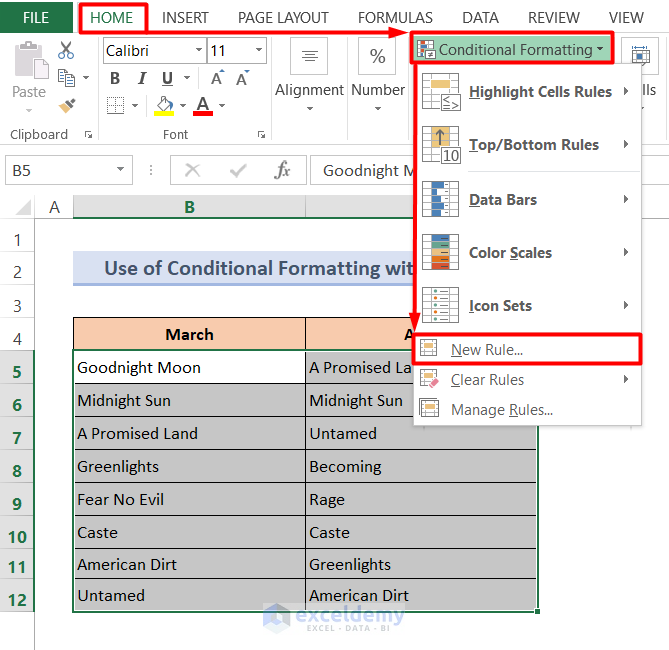
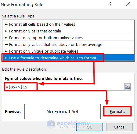
⏩Select Use a formula to determine which cells to format from the Select a Rule Type box.

⏩Enter the following formula in the Format values where this formula is true box:

⏩Click Format. The ‘Format Cells’ dialog box will appear.

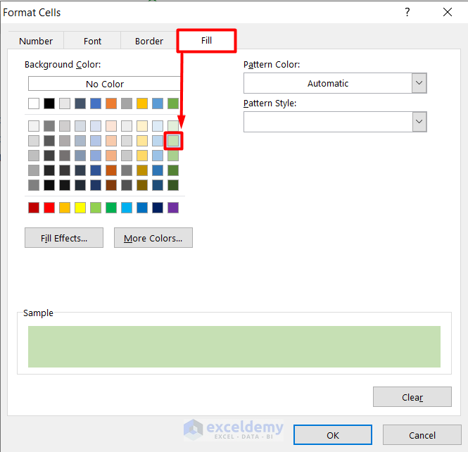
⏩Choose your desired color from the Fill tab. Here, light green.

⏩Click OK to return to the previous dialog box.

⏩Click OK.

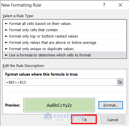
All the cells with different values in the same row are highlighted with the selected color.

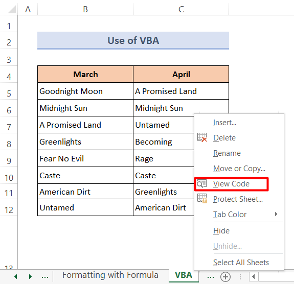
Method 5 – Using Excel VBA Macros

Instead of using built-in functions, we can use VBA code in Excel to highlight differences in the same row.

Steps:

⏩Right-click your mouse on the sheet title to open the VBA window.

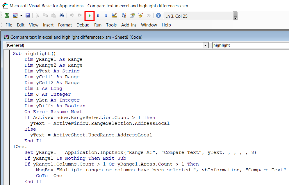
⏩Enter the following code into the box:

Sub highlight()
    Dim yRange1 As Range
    Dim yRange2 As Range
    Dim yText As String
    Dim yCell1 As Range
    Dim yCell2 As Range
    Dim I As Long
    Dim J As Integer
    Dim yLen As Integer
    Dim yDiffs As Boolean
    On Error Resume Next
    If ActiveWindow.RangeSelection.Count > 1 Then
      yText = ActiveWindow.RangeSelection.AddressLocal
    Else
      yText = ActiveSheet.UsedRange.AddressLocal
    End If
lOne:
    Set yRange1 = Application.InputBox("Range A:", "Compare Text", yText, , , , , 8)
    If yRange1 Is Nothing Then Exit Sub
    If yRange1.Columns.Count > 1 Or yRange1.Areas.Count > 1 Then
        MsgBox "Multiple ranges or columns have been selected ", vbInformation, "Compare Text"
        GoTo lOne
    End If
lTwo:
    Set yRange2 = Application.InputBox("Range B:", "Compare Text", "", , , , , 8)
    If yRange2 Is Nothing Then Exit Sub
    If yRange2.Columns.Count > 1 Or yRange2.Areas.Count > 1 Then
        MsgBox "Multiple ranges or columns have been selected ", vbInformation, "Compare Text"
        GoTo lTwo
    End If
    If yRange1.CountLarge <> yRange2.CountLarge Then
       MsgBox "Two selected ranges must have the same numbers of cells ", vbInformation, "Compare Text"
       GoTo lTwo
    End If
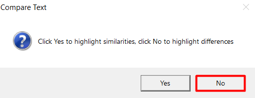
    yDiffs = (MsgBox("Click Yes to highlight similarities, click No to highlight differences ", vbYesNo + vbQuestion, "Compare Text") = vbNo)
    Application.ScreenUpdating = False
    yRange2.Font.ColorIndex = xlAutomatic
    For I = 1 To yRange1.Count
        Set yCell1 = yRange1.Cells(I)
        Set yCell2 = yRange2.Cells(I)
        If yCell1.Value2 = yCell2.Value2 Then
            If Not yDiffs Then xCell2.Font.Color = vbRed
        Else
            yLen = Len(yCell1.Value2)
            For J = 1 To yLen
                If Not yCell1.Characters(J, 1).Text = yCell2.Characters(J, 1).Text Then Exit For
            Next J
            If Not yDiffs Then
                If J <= Len(yCell2.Value2) And J > 1 Then
                    yCell2.Characters(1, J - 1).Font.Color = vbRed
                End If
            Else
                If J <= Len(yCell2.Value2) Then
                    yCell2.Characters(J, Len(yCell2.Value2) - J + 1).Font.Color = vbRed
                End If
            End If
        End If
    Next
    Application.ScreenUpdating = True
End Sub

⏩Press the Run button to run the code.

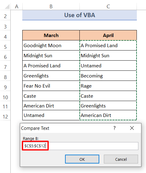
⏩A dialog box opens to select the first data range. Select the range B5:C12.

⏩Click OK. Another dialog box opens to select the second data range.

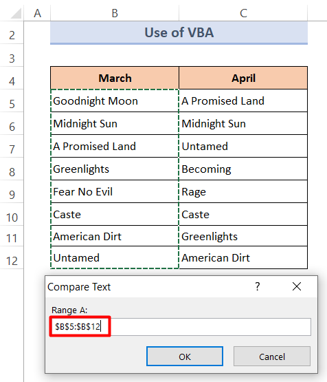
⏩Select the range C5:C12.

⏩Press OK again.

⏩To highlight differences, click No.

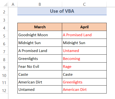
Different text in the same row is highlighted in red.

3 Quick Ways to Compare Text in Excel and Highlight Differences for All Rows

Method 1 – Using Conditional Formatting

Steps:

⏩Select the data range B5:C12.

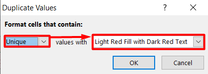
⏩Click Home > Conditional Formatting > Highlight Cells Rules > Duplicate Values.

A dialog box opens.

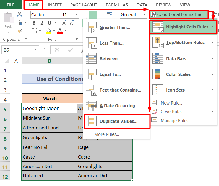
⏩Select the Unique option and desired color from the Format cells that contain box.

⏩Click OK.

All the different texts are now highlighted in our selected color.

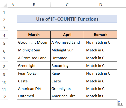
Method 2 – Using IF + COUNTIF Functions

Here, we’ll check whether the text of Column B can be matched anywhere in Column C, not just in the same row as previously.

The IF function checks whether a condition is met and returns one value if true and another if false. COUNTIF is used to count cells in a range that meet a single condition.

Steps:

⏩Enter the following formula in Cell D5:

⏩Press Enter.

⏩Drag the Fill Handle to copy the combined formula down to cell D12.

The results are as follows:

⏬ Formula Breakdown:

➥ COUNTIF($C$5:$C$12,$B5)=0

The COUNTIF function runs through the range C5:C12 and checks for matches with the contents of Cell B5. If no matches are found it returns FALSE, else it returns the number of matches found.

➥ IF(COUNTIF($C$5:$C$12,$B5)=0,”No match in C”,”Match in C”)

The IF function displays ‘No match in C’ for FALSE and ‘Match in C’ if not FALSE.

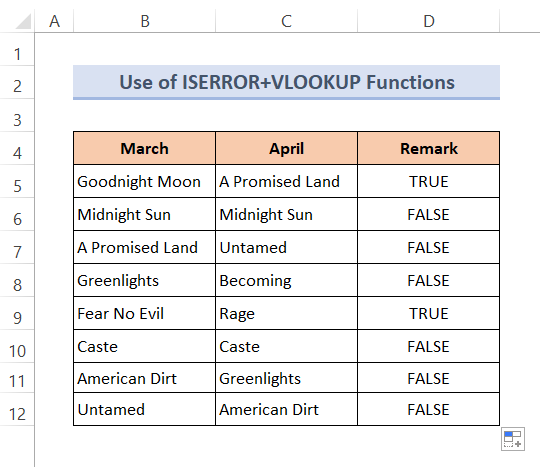
Method 3 – Using ISERROR + VLOOKUP Functions

This method will check the text in Column B for matches in Column C. Unmatched text will return TRUE and matched text FALSE.

The ISERROR function checks whether a value is an error and returns either TRUE or FALSE.

The VLOOKUP function is used to look up a value in the leftmost column of a table and return the corresponding value from a column to the right.

Steps:

⏩Enter the following formula in Cell D5:

⏩Press Enter and use the Fill Handle tool to copy the formula.

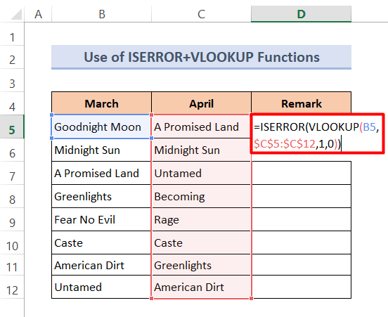
The output is as follows:

⏬ Formula Breakdown:

➥ VLOOKUP(B5,$C$5:$C$12,1,0)

The VLOOKUP function will check Cell B5 for matches in the range C5:C12. If it finds a matched value then it will return that value else it will return #N/A.

The result for Cell B5:

#N/A

➥ ISERROR(VLOOKUP(B5,$C$5:$C$12,1,0))

The ISERROR function will show “TRUE” for the result #N/A and “FALSE” for other outputs.

For Cell B5 it will return:

“TRUE”

Download Practice Book

<< Go Back To Excel Compare Cells | Compare in Excel | Learn Excel