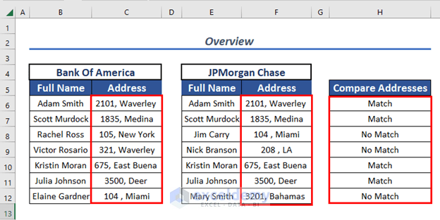
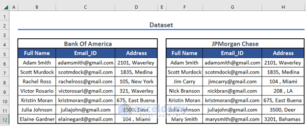
To demonstrate our methods, we’ll use the following dataset of two sets of bank customers, and find out which have accounts at both banks.
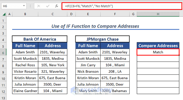
Method 1 – Using the IF Function
Steps:
- Select any cell to place your resultant value. Here, cell H5.
- Enter the following formula in the selected cell or in the Formula Bar:
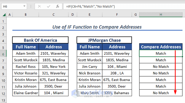
=IF(C6=F6,"Match","No Match")
- Press ENTER to return the output.
Formula Explanation
- The IF function checks whether the value of the selected cells are equal or not.
- If it is, it will return Match otherwise Not Match.
- Ue the Fill Handle to AutoFill the formulas for the rest of the cells.
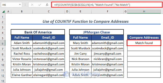
Method 2 – Using IF & COUNTIF Functions
Here, we will compare the Email_ID of the two sets of customers.
Steps:
- In cell H6, enter the following formula:
=IF(COUNTIF($C$6:$C$12,F6)>0, "Match Found","No Match")
- Press ENTER to return the output.
Formula Breakdown
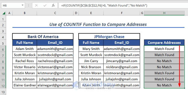
- COUNTIF($C$6:$C$12,F6)>0 → The logical statemen will be TRUE if F6 occurs multiple times in the range C6:C12.
- Output: TRUE
- IF(COUNTIF($C$6:$C$12,F6)>0, “Match Found”,”No Match”) → This becomes:
- IF(TRUE, “Match Found”,”No Match”)
- Output: Match Found
- Use the Fill Handle to AutoFill the formulas for the rest of the cells in column H.
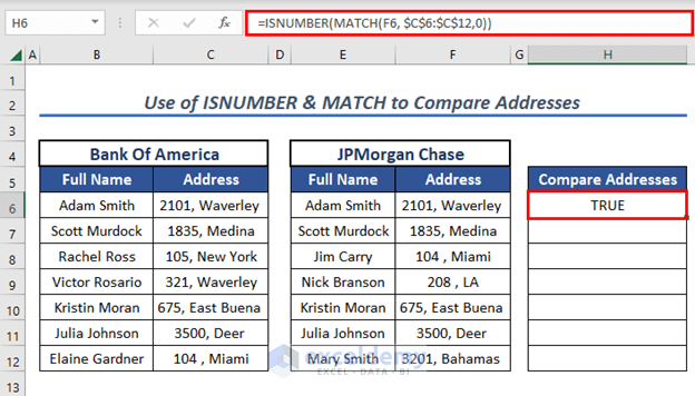
Method 3 – Combining ISNUMBER & MATCH Functions
Steps:
- In cell H6, enter the following formula:
=ISNUMBER(MATCH(F6,$C$6:$C$12,0))
- Press ENTER to return the output.
Formula Breakdown
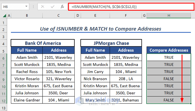
- MATCH(F6, $C$6:$C$12,0) → F6 is the lookup_value and C6:C12 is the lookup_array with match_type 0
- Output: 1
- ISNUMBER(MATCH(F6, $C$6:$C$12,0)) → This becomes:
- ISNUMBER(1)
- Output: TRUE
- Use the Fill Handle to AutoFill the formulas for the rest of the cells.
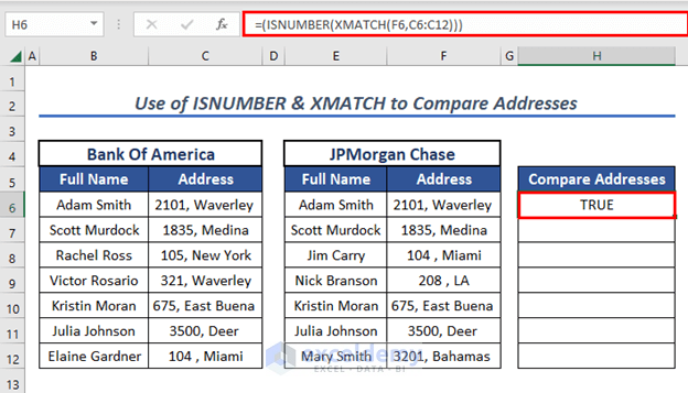
Method 4 – Merging ISNUMBER & XMATCH Functions
Both the ISNUMBER function and the XMATCH function are only available in Microsoft 365.
Steps:
- In cell H6, enter the following formula:
=(ISNUMBER(XMATCH(F6,C6:C12)))
- Press ENTER to return the output.
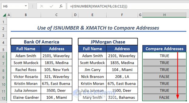
- Use the Fill Handle to AutoFill the formulas for the rest of the cells.
Formula Breakdown
- XMATCH(F6, C6:C12,0) → F6 cell is the lookup_value and C6:C12 is the lookup_array with match_type 0.
- Output: 1
- ISNUMBER(XMATCH(F6, C6:C12,0)) → This becomes:
- ISNUMBER(1)
- Output: TRUE
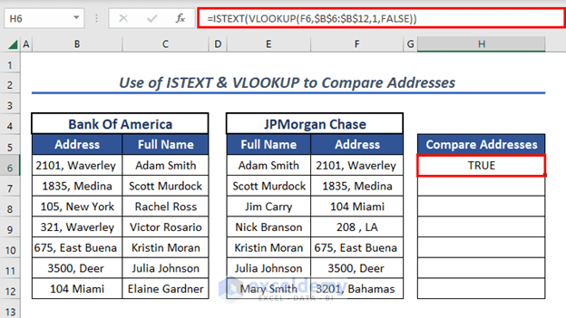
Method 5 – Combining ISTEXT & VLOOKUP Functions
Steps:
- In cell H6, enter the following formula:
=ISTEXT(VLOOKUP(F6,$B$6:$B$12,1,FALSE))
- Press ENTER to return the output.
Formula Breakdown
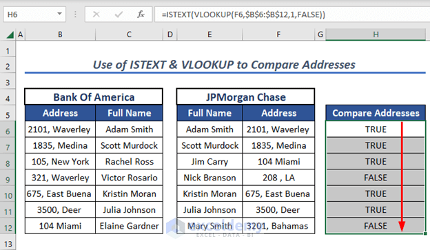
- VLOOKUP(F6,$B$6:$B$12,1,FALSE) → F6 is the lookup_value, C6:C12 is the table_array, the col_index_num is 1 and the range_lookup is FALSE.
- Output: “2101, Waverley “
- ISTEXT(VLOOKUP(F6,$B$6:$B$12,1,FALSE)) → This becomes:
- ISTEXT(“2101, Waverley “)
- Output: TRUE
- Use the Fill Handle to AutoFill the formulas for the rest of the cells.
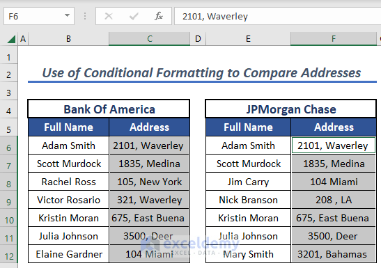
Method 6 – Using Conditional Formatting
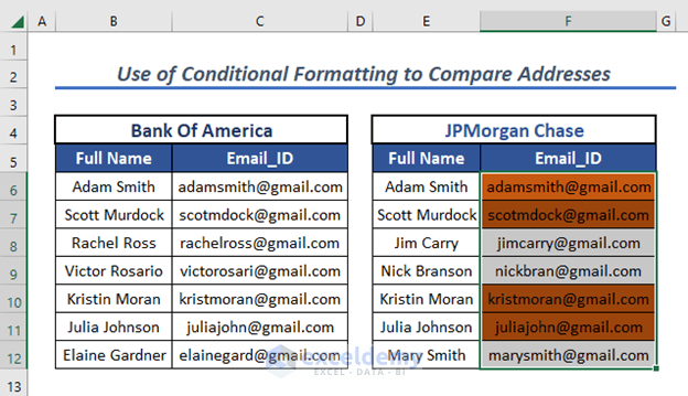
In addition to the use of functions, we can use Conditional Formatting to compare addresses by highlighting the matched values.
Steps:
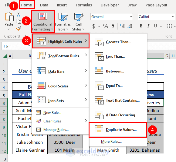
- Select the cell range. Here, we select two columns by selecting the first, holding the CTRL key, then selecting the second.
- Open the Home tab >> go to Conditional Formatting >> select Highlight Cells Rules >> select Duplicate Values.
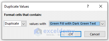
A Duplicate Values dialog box will pop up.
- Select Duplicate.
- Select the colors to highlight duplicate values. For example, the Green Fill with Dark Green Text.
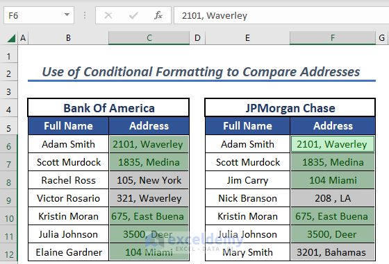
After clicking OK, the duplicate values in the two selected columns will be highlighted.
Method 7 – Using Conditional Formatting with Formula
We can use Conditional Formatting from the ribbon to compare addresses by using formulas.
Steps:
- Select the cell range, here column F.
- Open the Home tab >> go to Conditional Formatting >> select New Rule.
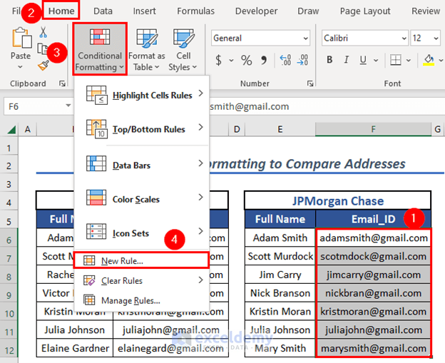
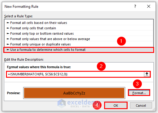
A New Formatting Rule dialog box will pop up.
- From Select a Rule Type select Use a formula to determine which cells to format.
- In Edit the Rule Description enter the following formula:
=ISNUMBER(MATCH(F6, $C$6:$C$12,0))
- Click Format and choose a color to fill the cells.
Formula Breakdown
- MATCH(F6, $C$6:$C$12,0) → F6 cell is the lookup_value and C6:C12 is the lookup_array with match_type 0.
- Output: 1
- ISNUMBER(MATCH(F6, $C$6:$C$12,0)) → This becomes:
- ISNUMBER(1)
- Output: TRUE
- Click OK.
The cells where the values are matched are filled with the selected format.
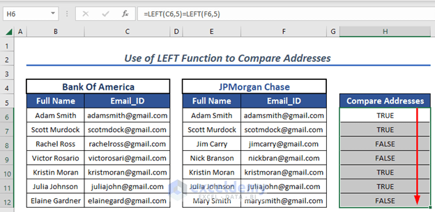
Method 8 – Using the LEFT Function
Steps:
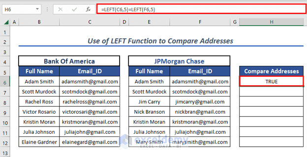
- In cell H6, enter the following formula:
=LEFT(C6,5)=LEFT(F6,5)
- Press ENTER.
The result of the address comparison between cells C6 and F6 is shown.
Formula Explanation
- The LEFT function checks whether the character of the selected cell is equal or not.
- We selected cell C6 as text and gave num_chars = 5.
- If the first 5 characters from the left of selected cell C6 match with the selected cell F6 then it will return TRUE otherwise FALSE
- Use the Fill Handle to AutoFill the formulas for the rest of the cells.
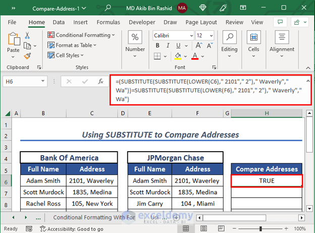
Method 9 – Using the SUBSTITUTE Function
We can use the SUBSTITUTE function combined with the LOWER function to compare addresses.
Steps:
- In cell H6, enter the following formula:
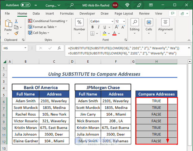
=(SUBSTITUTE(SUBSTITUTE(LOWER(C6)," 2101"," 2")," Waverly"," Wa"))=SUBSTITUTE(SUBSTITUTE(LOWER(F6)," 2101"," 2")," Waverly"," Wa")
- Press ENTER.
- The result of comparing the addresses in cells C6 and F6 is shown.
Formula Breakdown
- LOWER(C6) → This is the text for the SUBSTITUTE function.
- Output: “2101, waverley “
- SUBSTITUTE(LOWER(C6),” 2101″,” 2″) → This becomes:
- SUBSTITUTE(“2101, waverley”,” 2101″,” 2″)
- (SUBSTITUTE(SUBSTITUTE(LOWER(C6),” 2101″,” 2″),” Waverly”,” Wa”))=SUBSTITUTE(SUBSTITUTE(LOWER(F6),” 2101″,” 2″),” Waverly”,” Wa”) → This will compare the two addresses in C6 and F6.
- Output: TRUE
- Use the Fill Handle to AutoFill the formulas for the rest of the cells.
In most cases you may need to adjust the formula based on the cell values.
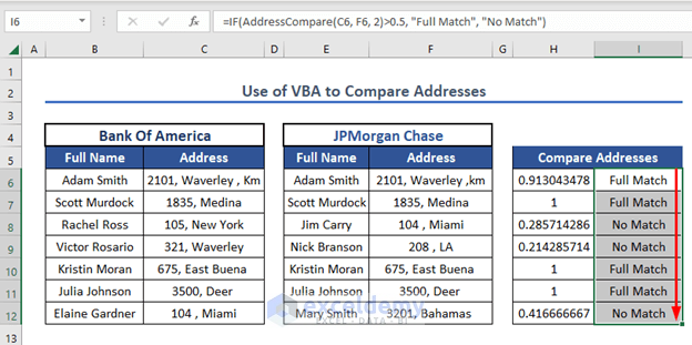
Method 10 – Using VBA Code
Steps:
- Press ALT + F11 to open the VBA window.
- Go to Insert >> select Module.
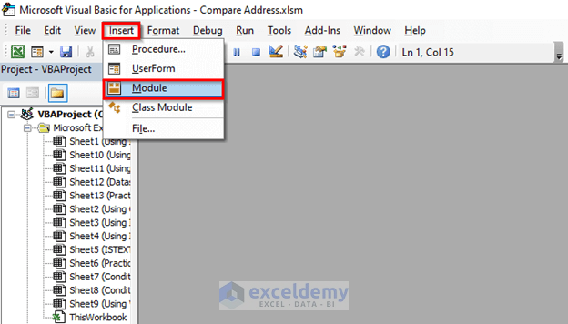
A new Module will open.
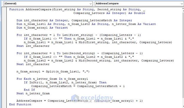
- Enter the following code to compare two addresses:
Function AddressCompare(first_string As String, Second_string As String, _
                                   Comparing_Letters As Integer) As Double
    Dim int_character As Integer, Comparing_LettersMatch As Integer
    Dim n_Gram_List1 As String, n_Gram_List2 As String, n_letter_Gram As Variant
    Dim n_Gram_array1 As Variant
    For int_character = 1 To Len(first_string) - (Comparing_Letters - 1)
        If n_Gram_List1 <> "" Then n_Gram_List1 = n_Gram_List1 & ","
        n_Gram_List1 = n_Gram_List1 & Mid(first_string, int_character, Comparing_Letters)
    Next int_character
    For int_character = 1 To Len(Second_string) - (Comparing_Letters - 1)
        If n_Gram_List2 <> "" Then n_Gram_List2 = n_Gram_List2 & ","
        n_Gram_List2 = n_Gram_List2 & Mid(Second_string, int_character, Comparing_Letters)
    Next int_character
    n_Gram_array1 = Split(n_Gram_List1, ",")
    For Each n_letter_Gram In n_Gram_array1
        If InStr(1, n_Gram_List2, n_letter_Gram) Then
            Comparing_LettersMatch = Comparing_LettersMatch + 1
        End If
    Next n_letter_Gram
    AddressCompare = Comparing_LettersMatch / (UBound(n_Gram_array1) + 1)
End Function
VBA Code Breakdown
- We create a new function named “AddressCompare”. The arguments are First_string, Second_string, and Comparing_Letters.
- We define some variables named int_character, Comparing_LettersMatch, n_Gram_List1, n_Gram_List2, n_letter_Gram, and n_Gram_array1
- We use a For_Loop.
- Save the code and go back to the worksheet.
- In cell H6, enter the following formula containing the function just created:
=AddressCompare(C6,F6,2)
- Press ENTER to return the output.
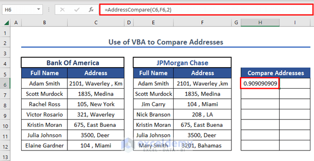
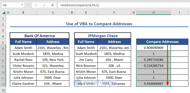
The AddressCompare function will compare how many characters of a text string match, and return the result as a numeric value where 1 represents a 100% match.
- AutoFill up to cell H12.
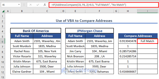
Now we can use the IF function to represent these numeric values as Text.
- In cell I6, enter the following formula:
=IF(AddressCompare(C6, F6, 2)>0.5, "Full Match", "No Match")
- Press ENTER.
The results of the address comparisons are displayed as text values, not numbers.
Formula Explanation
- The IF function checks if the matched value is greater than 0.5.
- If true, it will return Full Match else No Match.
- AutoFill up to cell I12.
Method 11 – Using Equal (=) Operator
We can use the simple equal operator (=) to compare addresses when the addresses are side by side in a row.
Steps:
- In cell H6, enter the following formula:
=C6=F6
- Press ENTER to return the output.
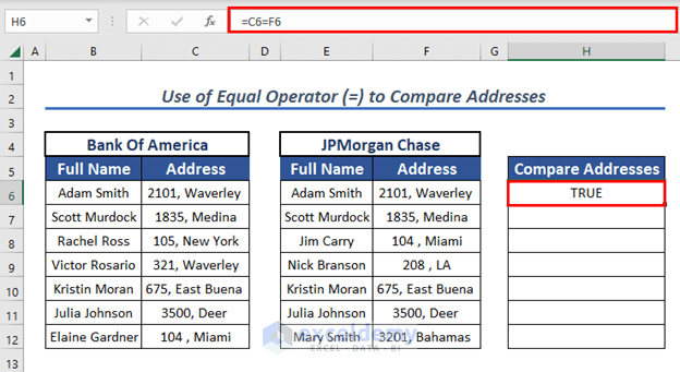
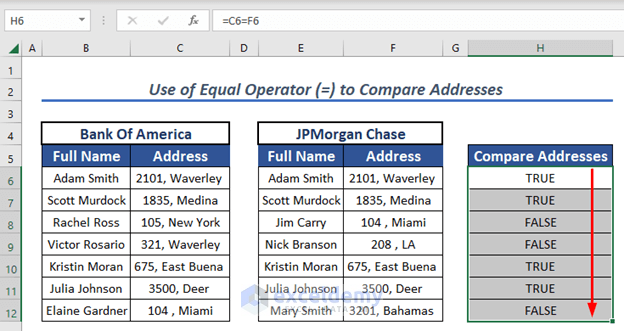
The equal operator will check whether both selected values are equal or not.
- Use Fill Handle to AutoFill the formulas for the rest of the cells.
Download to Practice Workbook
<< Go Back To Excel Compare Cells | Compare in Excel | Learn Excel
Get FREE Advanced Excel Exercises with Solutions!

Thanks for this VBA function; I added it in as a module, doublechecked my syntax, and still receive a #Name error. I modified my address lists to more closely match the examples and refreshed (running this in xlsm with macros enabled); still receive #NAME error. What am I doing wrong? Also, for a list with more than two variables (more like “5400 Menaul NE, Albuquerque, NM” vs “5400 Menaul Blvd NE, Albuquerque, NM”) would the last variable be 3 instead of 2?
Dear ABBY SHULER
Thank you for your comment. Here, for your first problem, to get rid of the #NAME error, you can copy the following VBA code in a new Excel Workbook. The uploaded Excel file sometimes show problem while running on a different computer, therefore, when you will copy the code to a new workbook, the #NAME error will be solved.
Function AddressCompare(first_string As String, Second_string As String, _
Comparing_Letters As Integer) As Double
Dim int_character As Integer, Comparing_LettersMatch As Integer
Dim n_Gram_List1 As String, n_Gram_List2 As String, n_letter_Gram As Variant
Dim n_Gram_array1 As Variant
For int_character = 1 To Len(first_string) – (Comparing_Letters – 1)
If n_Gram_List1 <> “” Then n_Gram_List1 = n_Gram_List1 & “,”
n_Gram_List1 = n_Gram_List1 & Mid(first_string, int_character, Comparing_Letters)
Next int_character
For int_character = 1 To Len(Second_string) – (Comparing_Letters – 1)
If n_Gram_List2 <> “” Then n_Gram_List2 = n_Gram_List2 & “,”
n_Gram_List2 = n_Gram_List2 & Mid(Second_string, int_character, Comparing_Letters)
Next int_character
n_Gram_array1 = Split(n_Gram_List1, “,”)
For Each n_letter_Gram In n_Gram_array1
If InStr(1, n_Gram_List2, n_letter_Gram) Then
Comparing_LettersMatch = Comparing_LettersMatch + 1
End If
Next n_letter_Gram
AddressCompare = Comparing_LettersMatch / (UBound(n_Gram_array1) + 1)
End Function
After that, save the code and go back to your worksheet. I hope the #NAME error will be gone now.
For your second query, you can use 3 instead of 2. Using 3 will compare 3 letters at a time, and therefore, the result will decrease the match percentage between two addresses.
When you will use 2, it will compare 2 letters at a time, and therefore, the match percentage between two addresses will be higher.
Let me show you that elaborately.
When we use
=AddressCompare(C5, F5, 2)in cell E3, the result becomes 1, which indicates the Exact Match.However, the two addresses are not the same, therefore, using 2 does not give an accurate result.
On the other hand, when we use the formula
=AddressCompare(C5, F5, 3)in cell E3, the result becomes 0.970588235, which does not indicate the Exact Match. Rather, it suggests that there is some dissimilarity between the two addresses.Therefore, using 3 is wise in your case.
Here, another thing must be noted, for your address match, you have to set your own creation while using the IF function.
Let me elaborate on this.
Here, in cell F3, we type the following formula.
IF(AddressCompare(C5, F5, 3)>0.5, "Full Match", "No Match")Here, in this formula, we give the criteria, that when AddressCompare(C5, F5, 2) is greater than 0.5, the IF function returns “Full Match“. However, when AddressCompare(C5, F5, 2) is not greater than 0.5, the IF function returns “No Match“.
Therefore, in cell F3 the result is “Full Match“.
However, there is some dissimilarity between the two addresses. Hence, the result in cell F3 is not accurate.
To get an accurate result, we will type the following formula in cell F3.
IF(AddressCompare(C5, F5, 3)>0.99, "Full Match", "No Match")Here, in this formula, we give the criteria, that when AddressCompare(C5, F5, 2) is greater than 0.99, the IF function returns “Full Match“. However, when AddressCompare(C5, F5, 2) is not greater than 0.99, the IF function returns “No Match“.
Therefore, in cell F3 the result is “No Match“.
This is the correct result.
I really hope that you get your answer, and that you can solve your problems.
If you face any problem, you can always let us know.
Regards,
Afia Aziz Kona