Compare Two Cells Using Conditional Formatting in Excel (3 Methods)

Excel has an amazing feature called Conditional Formatting that enables us to do a lot of things with our data in Excel. You can analyze your data in Excel by marking different values with the help of conditional formatting. In this article, you will learn 3 methods to compare two cells using conditional formatting in Excel.

Compare Two Cells Using Conditional Formatting in Excel: 3 Methods

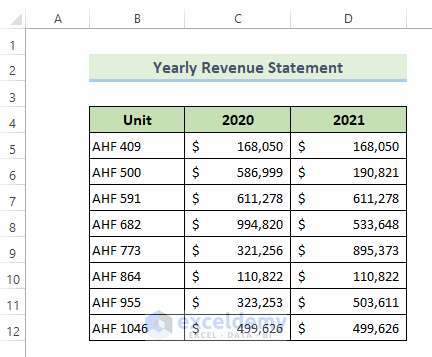
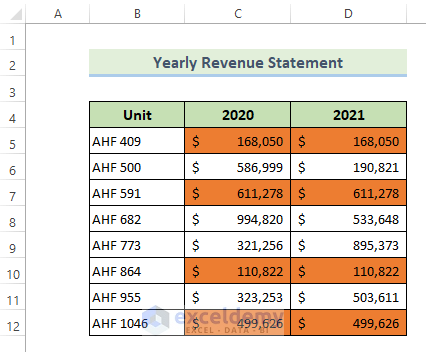
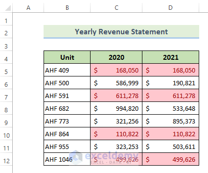
We have a dataset of  3 columns titled Yearly Revenue Statement.

The first column contains different unit names. The second and third column contains yearly revenues in dollars against the unit names.

1. Compare Two Cells Using Conditional Formatting to Highlight Matched Records in Excel

We will compare the values of the cells in between the second and the third column.

To do that,

❶ Select those two columns first and go to the Home tab.

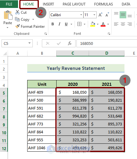
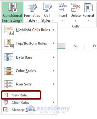
❷ After that click on the Conditional Formatting drop-down and choose New Rule from the drop-down list.

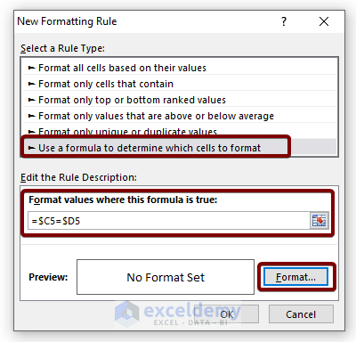
A New Formatting Rule dialog box will appear.

❸ Choose Use a formula to determine which cells to format from the Select a Rule Type section.

❹ Under the Format values where this formula is true section, enter the following formula:

This formula will compare whether cell C5 is equal to cell D5 or not.

❺ Then hit on the Format button.

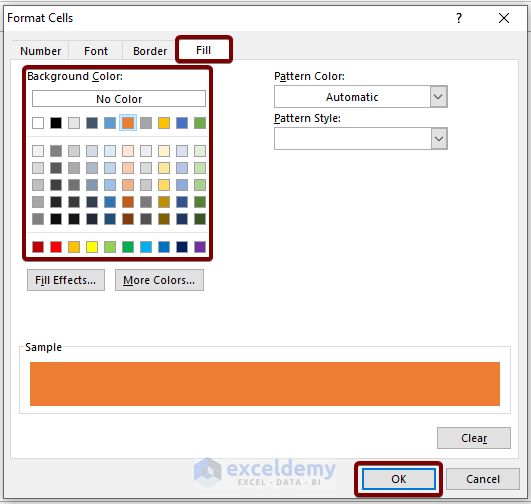
A Format Cells dialog box will appear.

❻ Go to the Fill tab.

❼ From the Background Color section, pick up a color.

❽ Finally hit the OK button.

This command will instantly highlight all the matched cells in between the second and the third columns.

2. Highlight Duplicates by Comparing Two Cells Using Conditional Formatting in Excel

To highlight all the duplicate cells without using a formula in the New Rule, follow the steps below:

❶ First select the cells where you want to run the comparison.

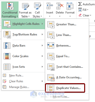
❷ Then go to the Home tab.

❸ After that go to Conditional Formatting > Highlight Cells Rules > Duplicate Values.

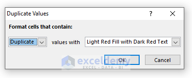
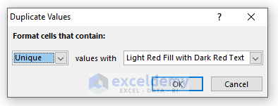
A Duplicate Values dialog box will appear.

❹ Select Duplicate in the Format cells that contain box.

❺ Select a color format in the values with box.

❻ Then hit OK.

After that you will see that all the cells with duplicates values have instantly highlighted with your selected color as in the picture below:

3. Compare and Highlight Unique Values from Two Cells Using Conditional Formatting

To compare two cells using the conditional formatting and highlight the unique values in Excel, follow the steps below:

❶ First select the cells where you want to run the comparison.

❷ Then go to the Home tab.

❸ After that go to Conditional Formatting > Highlight Cells Rules > Duplicate Values.

A Duplicate Values dialog box will appear.

❹ Select Unique in the Format cells that contain box.

❺ Select a color format in the values with box.

❻ Then hit OK.

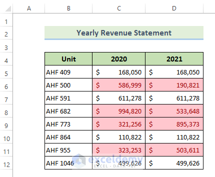
After that you will see that all the cells with unique values have instantly highlighted with your selected color as in the picture below:

Read More: How to Compare Text in Excel and Highlight Differences

Things to Remember

• Always make the cell selection first before applying the conditional formatting.

Download Practice Workbook

Conclusion

To sum up, we have discussed 3 methods to compare two cells using conditional formatting in Excel. You are recommended to download the practice workbook attached along with this article and practice all the methods with that. And don’t hesitate to ask any questions in the comment section below. We will try to respond to all the relevant queries ASAP.

<< Go Back To Excel Compare Cells | Compare in Excel | Learn Excel