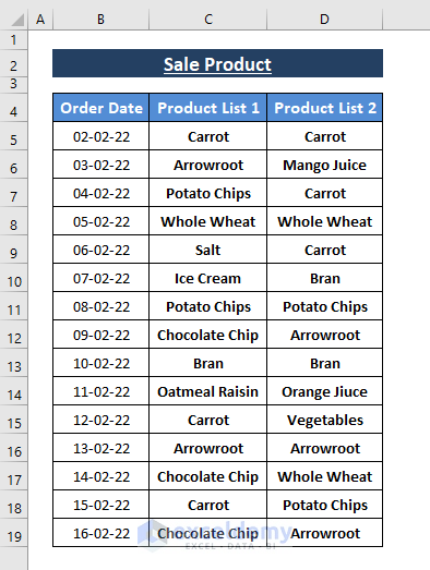
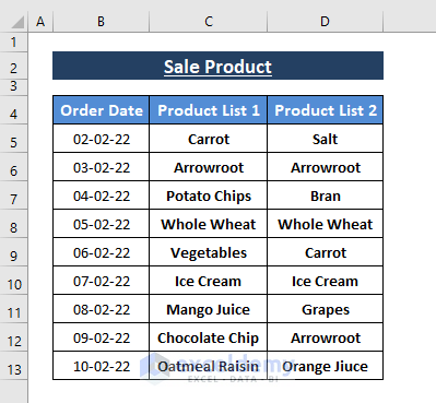
We have two different Product lists. The Product lists have products that are ordered on certain days. We want to compare these products on the same dates and color them if they are not identical.
How to Compare Two Cells and Change Their Color in Excel: 2 Ways
Method 1 – Using Conditional Formatting
Case 1.1 – Using Formula to Compare Cells and Change Colors
Steps:
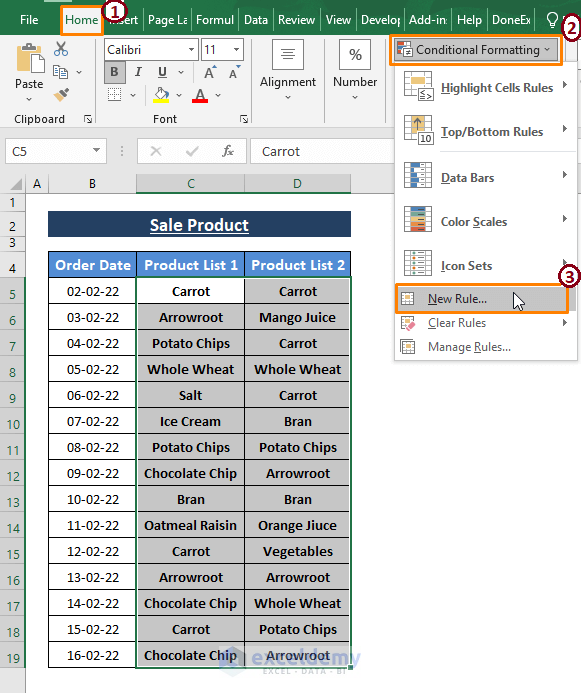
- Go to Home.
- Select Conditional Formatting (from the Style section).
- Choose New Rule (from the options).
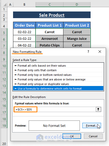
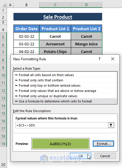
- The New Formatting Rule window appears.
- Select Use a formula to determine which cells to format.
- Enter the following formula in the Format values where this formula is a true field:
=$C5<>$D5The formula checks whether the entries (from row 5) in Column C and Column D are not equal. Then, conditional formatting changes the color of the cells if the formula returns TRUE.
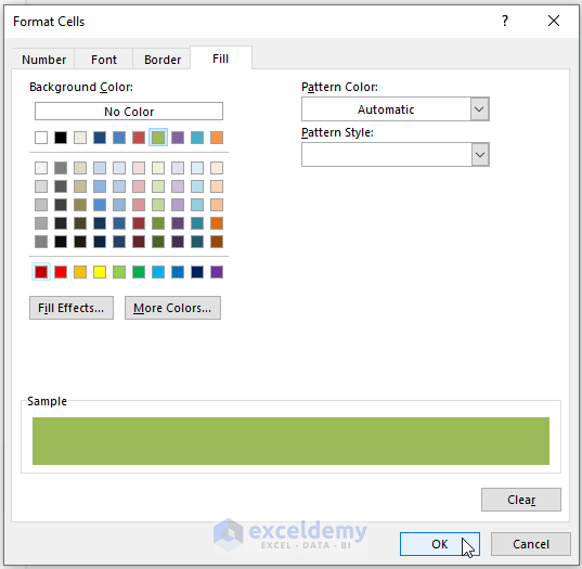
- Click on Format, which brings up the Format Cells window.
- Choose a Fill Color (i.e., Green).
- Click on OK.
- Click on OK.
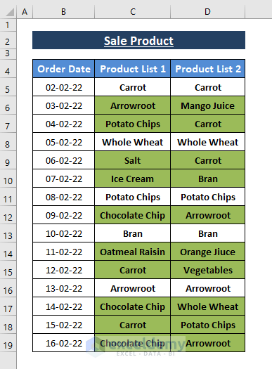
- All cells that satisfy the formula (i.e., $CX not equal to $DX) will be formatted.
Case 1.2 – Using Specific Cells to Compare and Format
- Follow the previous case and replace the formula in the Conditional Formatting Rule with the following:
- Click on OK.
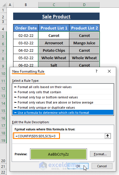
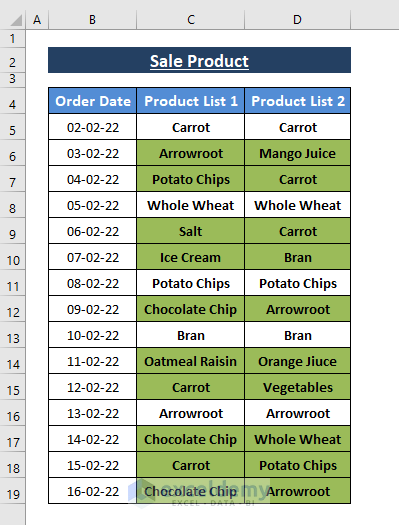
- You’ll get color-formatted values throughout the column.
You can modify the COUNTIF formula with your own range, criteria, and equal to values.
Case 1.3 – Using Unique Entries to Compare Cells and Color
We’ll modify the dataset to ensure we have Duplicate and Unique entries in both columns.
Steps:
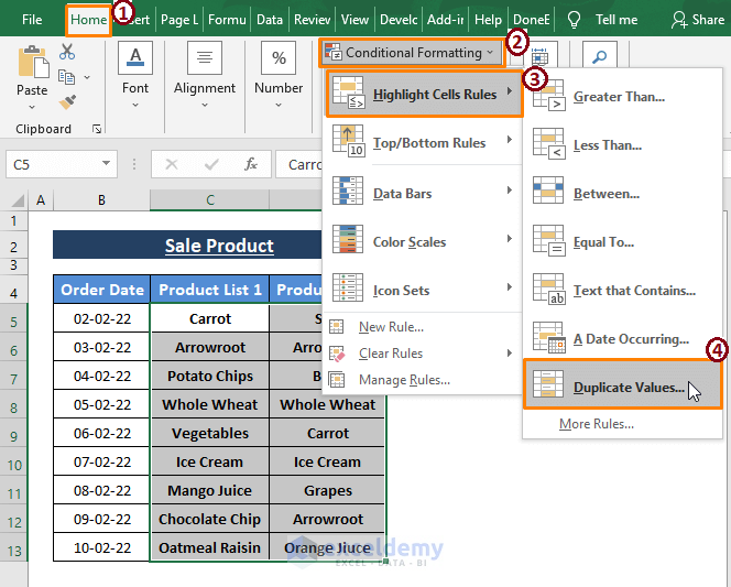
- In the Home tab, select Conditional Formatting (from the Style section).
- Click on Highlight Cells Rules.
- Select Duplicate Values (from the options).
- The Duplicate Values window appears.
- Select Unique values as Format cells that contain to color format cells.
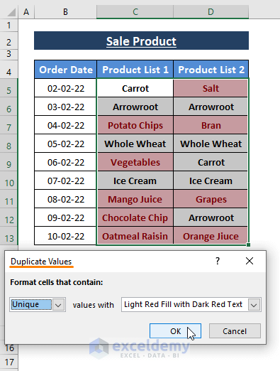
The Duplicate Values condition compares entries between two columns and color formats unique entries (throughout both columns).
Method 2 – Using Go To Special to Compare Two Columns and Change Color
Steps:
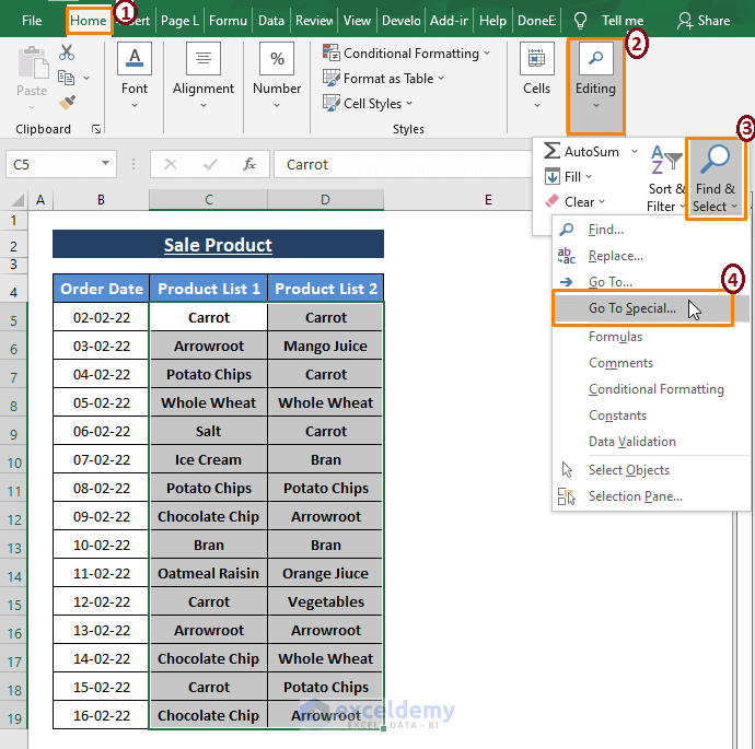
- In the Home tab, select Find & Select (from the Editing section.
- Choose Go To Special.
- The Go To Special dialog box appears.
- Choose Row Differences under the Select section.
- Click OK.
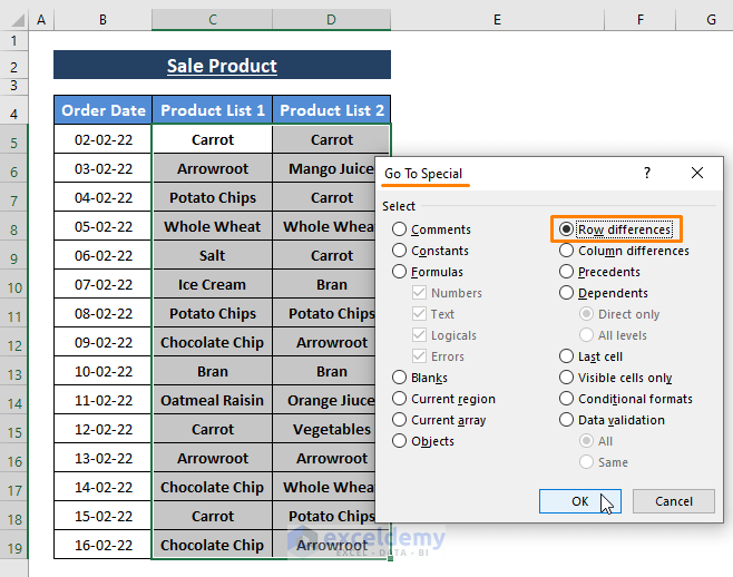
- Selecting Row Differences selects Unique entries of Column D comparing respective entries between Column C and D. The outcomes will be the same as shown in the following image.
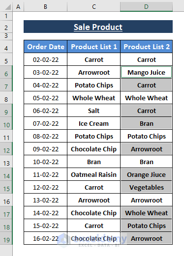
- In the Home tab, select a Fill Color (i.e., Theme Color) for the selected entries.
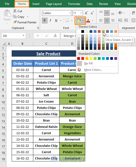
Go To Special’s Row Differences compares rows and selects the different entries that exist in the latter column. You can choose any theme color to format the selection. Changing the values doesn’t undo the formatting.
Download the Excel Workbook
<< Go Back To Excel Compare Cells | Compare in Excel | Learn Excel
Get FREE Advanced Excel Exercises with Solutions!
