Compare Two Cells in Excel and Return TRUE or FALSE (5 Quick Ways)

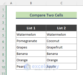
Let’s consider a dataset (B5:D10) containing fruit names in two columns (columns B and C). We will compare fruit names between these columns and return TRUE or FALSE accordingly.

Method 1 – Use the ‘Equal to’ Sign to Compare Two Cells and Return TRUE or FALSE

Steps:

• Use the below formula in Cell D5 and press Enter.

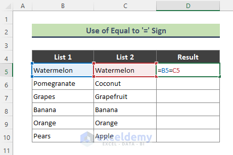
• Use the Fill Handle (+) tool to copy the formula to compare the rest of the cells.

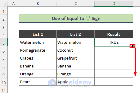
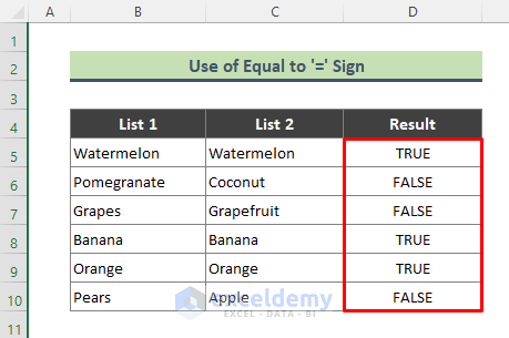
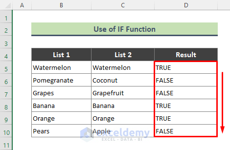
• Here’s the result.

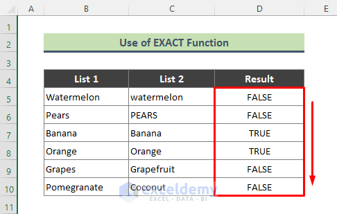
Method 2 – Compare Two Cells and Return TRUE or FALSE with the EXACT Function

Steps:

• Use the below formula in Cell D5 and hit Enter.

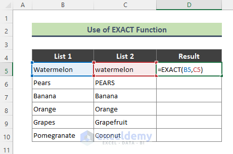
• Use the Fill Handle tool to copy the formula over the range D6:D11.

Method 3 – The Excel COUNTIF Function to Compare Two Cells and Get TRUE/FALSE

Steps:

• Use the following formula in Cell D5 and press Enter.

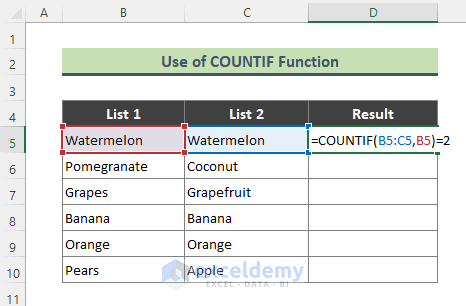
• Use the Fill Handle tool to copy the formula and compare the rest of the cells.

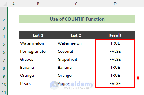
The COUNTIF function counts the number of cells within the range B5:C5, for the given condition B5:C10=B5. If there are exactly two cells that share a value of B5 (including B5), the formula returns TRUE. Since the range is composed of two cells (the cell in column B and its corresponding value in column C), that will only happen if the values are equal.

Method 4 – Use the IF Function to Compare Two Cells and Return TRUE or FALSE in Excel

Steps:

• Use the below formula in Cell D5 and hit Enter.

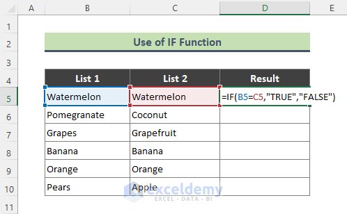
• Use the Fill Handle tool to copy the formula to the rest of the cells.

Method 5 – Combine VLOOKUP and ISERROR Functions to Compare Two Cells and Ignore Errors

Steps:

• Use the below formula in Cell D5 and press Enter.

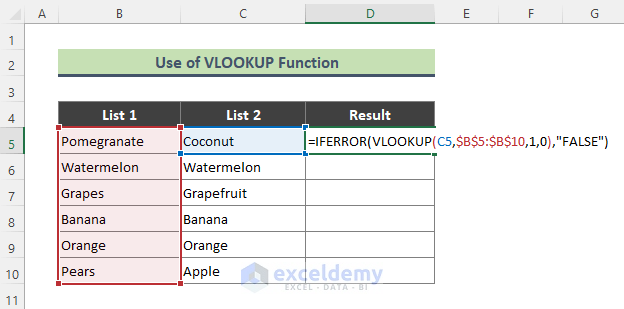
• Use the Fill Handle tool to compare other cells in the dataset.

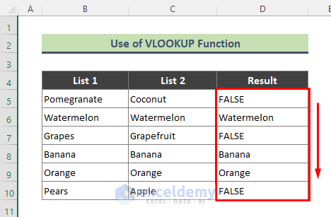
How Does the Formula Work?

• (VLOOKUP(C5,$B$5:$B$10,1,0)

The VLOOKUP function looks for the value of Cell B5 in the range B5:B10 returns:

{#N/A}

• IFERROR(VLOOKUP(C5,$B$5:$B$10,1,0),”FALSE”)

To avoid the error, we wrapped the VLOOKUP formula with the IFERROR function, and the formula returns:

{FALSE}

Download the Practice Workbook

<< Go Back To Excel Compare Cells | Compare in Excel | Learn Excel