While working in Microsoft Excel sometimes you might need to find the percentage of two numbers in Excel. This is often determined to calculate the difference between two values by using the division formula. Today in this article, I am sharing with you how to find the percentage of two numbers in Excel. Stay tuned!
In the following, I have shared 3 simple and easy methods to find the percentage of two numbers in Excel.
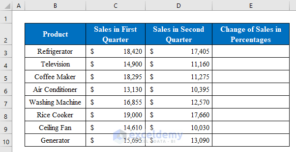
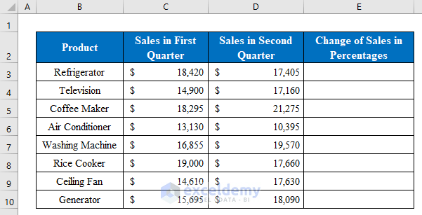
Suppose we have a dataset of some Products, Sales in the First Quarter, and Sales in the Second Quarter. Now we will calculate the percentage of those two numbers in our Excel worksheet.
1. Using Excel Formula to Find Percentage of Two Numbers
If you are looking for a simple solution to calculate the percentage difference between two numbers in Excel, then you are at the right place. Using a simple division formula you can find the percentage within a moment. Follow the steps below-
Steps:
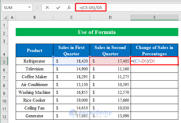
- First, choose a cell (E5) and apply the following formula-
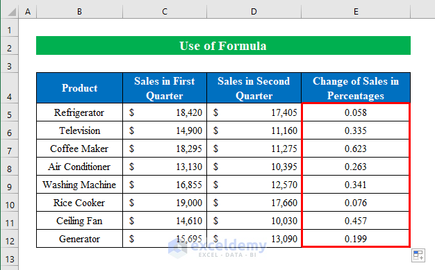
=(C5-D5)/D5- Second, Hit ENTER and drag the “Fill Handle” down to fill all the cells.
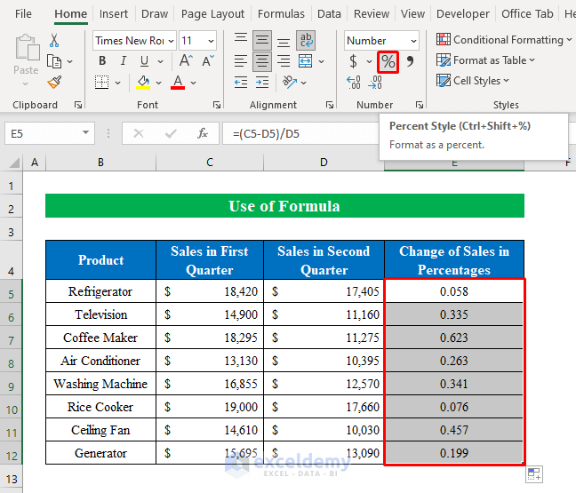
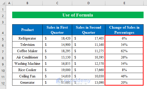
- Now, you will see the output is in decimal format. Let’s change them to percent style by choosing cells (E5:E12) and clicking the “Percent Style” icon from the Home
- That’s it. We have successfully found the percentage of two numbers in Excel within a glimpse of an eye.
2. Applying Keyboard Shortcut to Find the Percentage of Two Numbers
We always hunt for shortcuts to reach our destination quickly. Here, I am describing a keyboard shortcut to find the percentage of two numbers in Excel.
Steps:
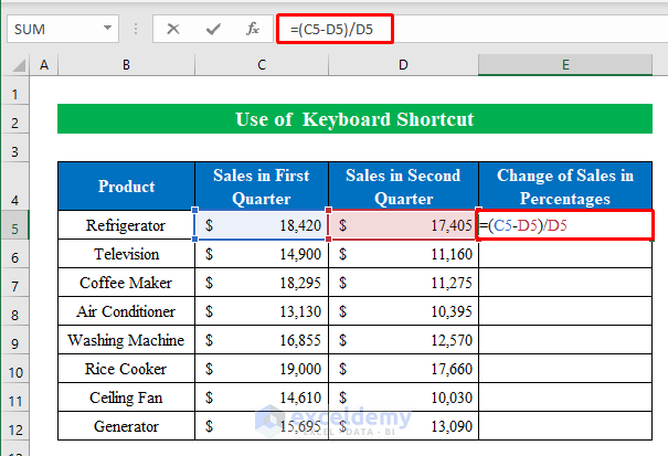
- In the same fashion, choose a cell (E5) and write the formula down-
=(C5-D5)/D5- Next, click ENTER and pull the “FillHandle” down.
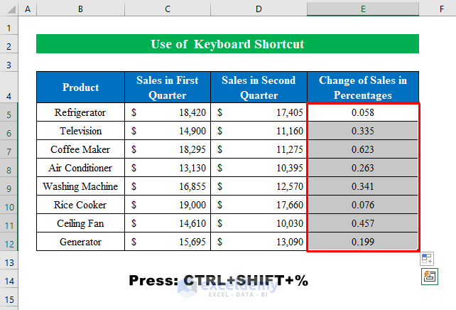
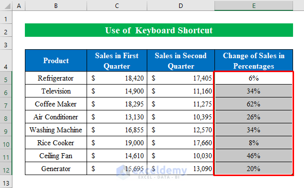
- While the output cells (E5:E12) are selected press CTRL+SHIFT+% from the keyboard.
- In summary, our result is ready in our hands with a simple shortcut.
3. Finding Percentage of Two Numbers in Different Excel Rows
Sometimes you might need to find the percentage of two numbers placed in the same column but in a different row. In that case, you can follow the below instructions.
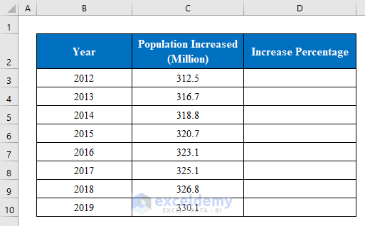
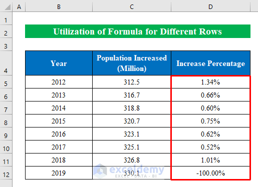
Suppose we have a dataset of some Yearwise Population Increased numeric Value. Now we will find the increased percentage yearly.
Steps:
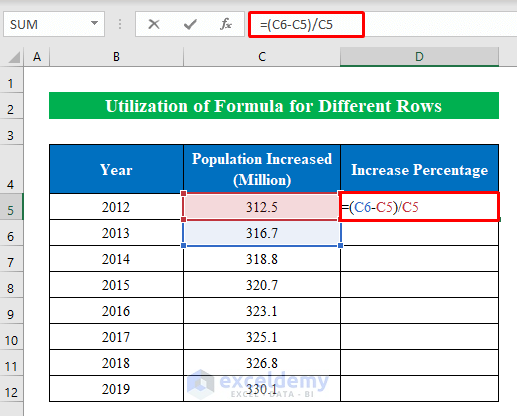
- To start with, select a cell (D5) and put the below formula down-
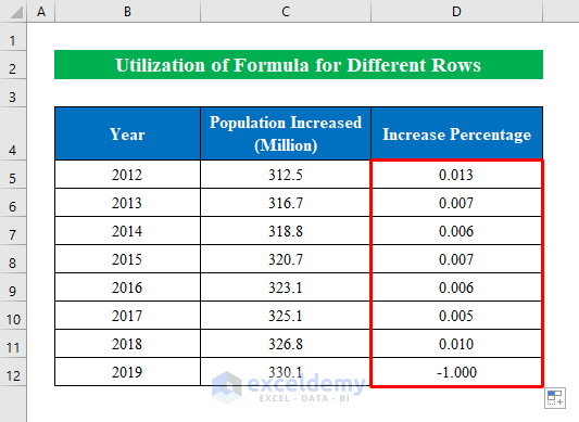
=(C6-C5)/C5- Gently, hit ENTER and drag down the “Fill Handle” to fill all the cells with the proper output.
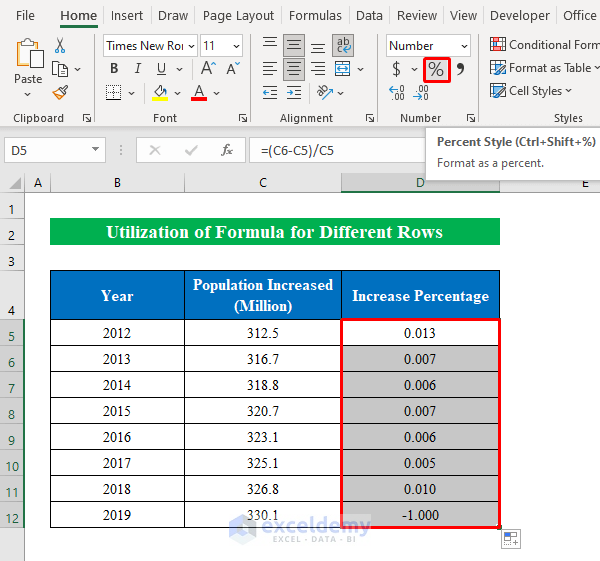
- Thereafter, selecting cells (D5:D12) change the style to “Percent Style” by hitting the “Percent” icon from the top ribbon.
- Finally, we have found the percentage of two numbers for different rows.
Finding Updated (Increment or Decrement) Numbers from Percentage in Excel
Often we need to determine the updated increased or decreased numbers from percentage values. Here, I will explain both numbers from percentages in an Excel worksheet.
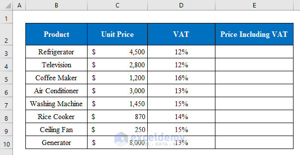
Imagine we have a dataset of some Products, Unit Prices, and VAT. Now we will calculate the Final Price using the percentage value in our workbook.
Steps:
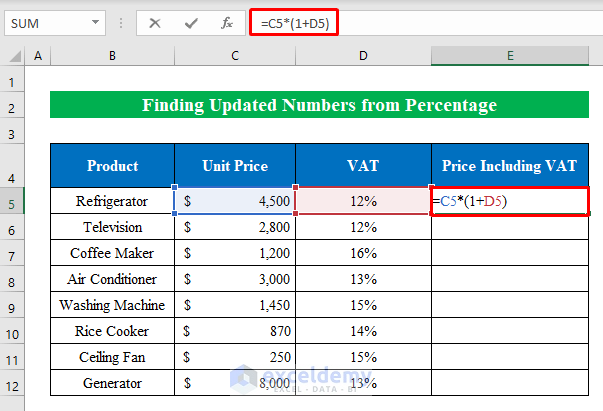
- Presently, choose a cell (E5) and apply the following formula-
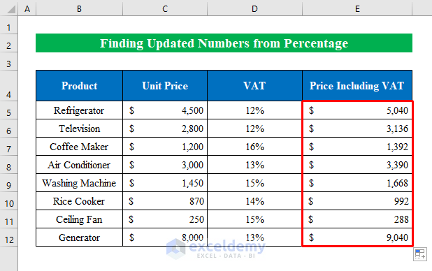
=C5*(1+D5)- Similarly, hit ENTER and drag down the “Fill Handle”.
- Hence, we got our increment output from the percentage value.
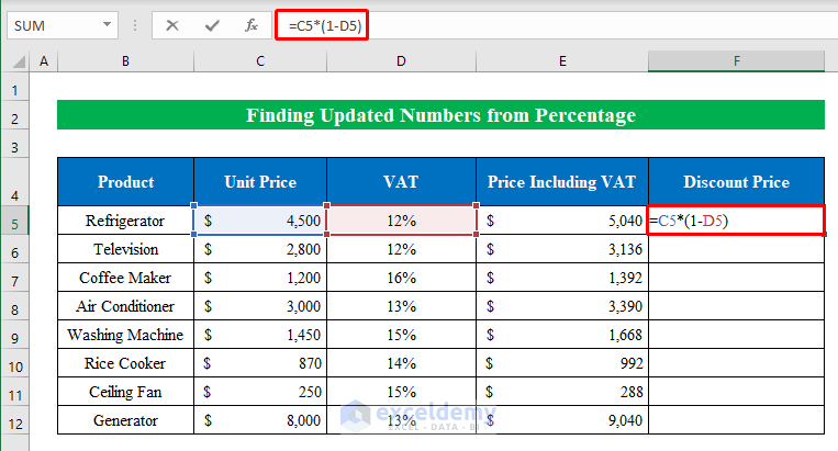
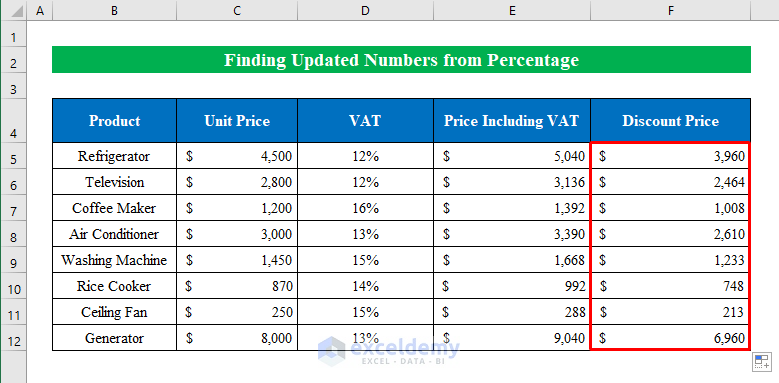
- Thereafter, to find the updated decreased value with percentage, we will choose a cell (F5) and write the formula inside the cell-
=C5*(1-D5)- In the same order, click ENTER and fill down the cells by dragging the “Fill Handle”.
- Finally, we have our decreased output in our hands.
Use Format Cells Feature to Mark Percentages of Two Numbers
For calculation advantage, you can mark the percentages the way you want by utilizing the format cells feature.
Suppose we have a dataset of some Products, Sales in the First Quarter, and Sales in the Second Quarter. Now we will calculate the Change of Sales and mark them according to our choice.
Steps:
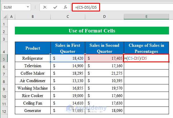
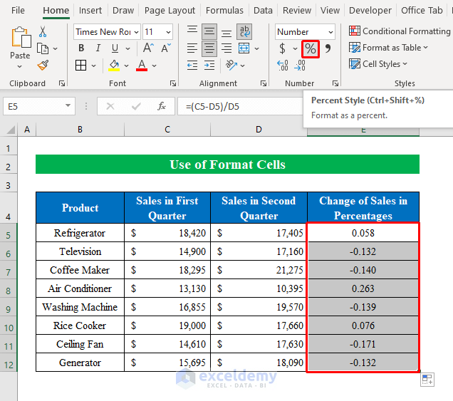
- First, choose a cell (E5) and apply the following formula-
=(C5-D5)/D5- Finish by, pressing ENTER and dragging the “Fill Handle” down.
- While the output is selected click the “Percent Style” icon from the top ribbon.
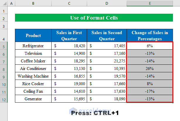
- As you can see, we have got our output in percentages.
- Hence, choosing all output results press CTRL+1 to go to the “Format Cells” window.
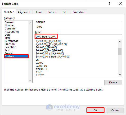
- In the new window, choose “Custom” and type “00%;[Red]-0.00%”.
- Thereafter, press OK.
- In conclusion, we have successfully marked all the negative percentage values in red. This is the simplest way to mark percentages. Simple isn’t it?
Download Practice Workbook
Download this practice workbook to exercise while you are reading this article.
Conclusion
In this article, I have tried to cover all the methods to find the percentages of two numbers in Excel. Take a tour of the practice workbook and download the file to practice by yourself. I hope you find it helpful. Please inform us in the comment section about your experience.
Related Articles
- How to Calculate Total Percentage from Multiple Percentages in Excel
- How to Calculate Percentage of Month in Excel
- How to Calculate Percentage of Percentage in Excel
- How to Calculate Percentage Based on Conditional Formatting
- How to Calculate Percentage in Excel Based on Cell Color
- Percentage Showing as Thousand in Excel
- Why Are My Percentages Wrong in Excel?
- How to Remove Percentage in Excel
- How to Calculate Percentage Complete Based on Dates in Excel
- How to Calculate Error Percentage in Excel
- How to Calculate Cumulative Percentage in Excel
<<Go Back to Calculating Percentages in Excel | How to Calculate in Excel | Learn Excel
Get FREE Advanced Excel Exercises with Solutions!