While working with Microsoft Excel, you may have dealt with several sheets in your workbook. However, if you need to create a table of contents with the sheet names, you can utilize the formulas. Today, in this article, we’ll learn six quick and suitable ways to make a table of contents without VBA in Excel effectively with appropriate illustrations.
How to Create Table of Contents Without Excel VBA: 6 Suitable Ways
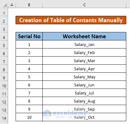
In the following figure, you see that we have 10 sheets which are mainly salaries in months along a year. Also, the names of the sheets are like Salary_Jan, Salary_Feb, and so on. Unfortunately, there is no dedicated function to get the list of sheet names in Excel. So we have to use the combination of several functions or the 2-step process of using Name Manager & formula. Here’s an overview of the dataset for today’s task.

1. Create Table of Contents Manually in Excel
In this section, we will create a table of contents manually without VBA. This is the easiest way. Let’s follow the instructions below to learn!
Step 1:
- First of all, select cell B5 and type the name of the worksheet manually in that cell. The names of the sheets are like Salary_Jan, Salary_Feb, and so on.
- As a result, you will be able to create a table of contents manually without VBA which has been given in the below screenshot.
Step 2:
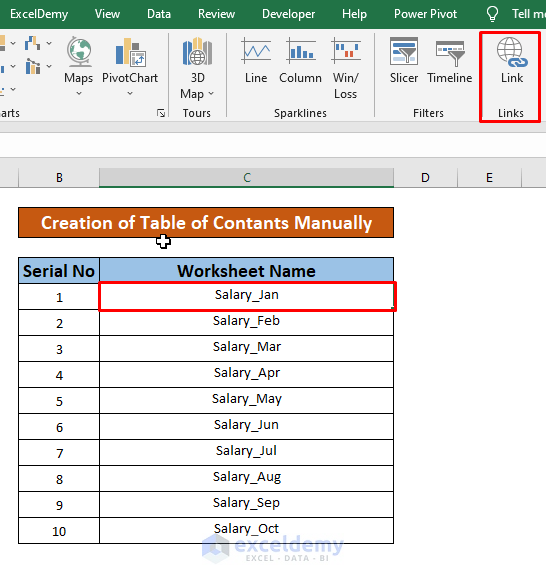
- Now we will link our cells with respect to their worksheets. To do this, click on cell C5, go to the Insert Tab and click on Link Option.
- From Insert Hyperlink Tab, select the desired excel file.

- Click Ok and then select Place in this Document. Then select Salary_Jan to continue.

- Click OK and our linking is done.

- Similarly, do the same process for all the cells.

Step 3:
- Click on any of the cells and it will take you to the respected worksheet.

- And our job is done!

Read More: How to Create Table of Contents Automatically in Excel
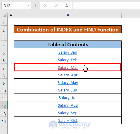
2. Combination of INDEX & FIND Functions to Create Table of Contents
If you want to create a table of contents with the sheet names using several functions, you may use the formula containing the INDEX, LEFT, MID, and FIND functions. Let’s follow the instructions below to learn!
Step 1:
- First of all, from your Formulas ribbon, go to,
Formulas → Defined Names → Name Manager
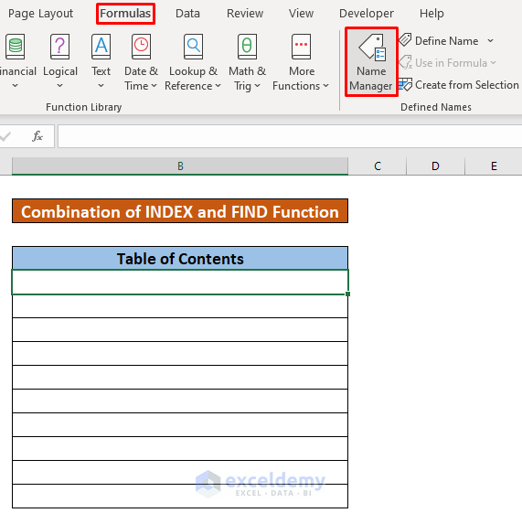
- As a result, a New Manager dialog box will appear in front of you. From the New Manager dialog box, select the New option.

- Hence, a New Name pops up. From the New Name dialog box, insert the Name (here the name is Worksheets) and the below formula in the Refers to section.
=GET.WORKBOOK(1) & T(NOW())
Step 2:
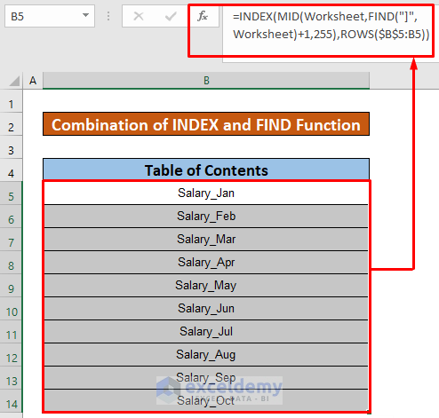
- After that, enter the following formula in the B5 cell where you want to get the sheet names.
=INDEX(MID(Worksheet,FIND("]",Worksheet)+1,255),ROWS($B$5:B5))
- Finally, if you press Enter and use Fill Handle Tool for the below cells, you’ll create a table of contents of sheet names like the following.
Read More: How to Create Table of Contents for Tabs in Excel
3. Apply INDEX Function Along with REPLACE Function to Create Table of Contents
Again, you can insert the below formula in the Refers to section and the Name as SheetsName after clicking the New option from the Name Manager dialog box. Let’s follow the instructions below to learn!
Step 1:
- Write down the below formula in the Refers to section.
=REPLACE(GET.WORKBOOK(1),1,FIND("]",GET.WORKBOOK(1)),"")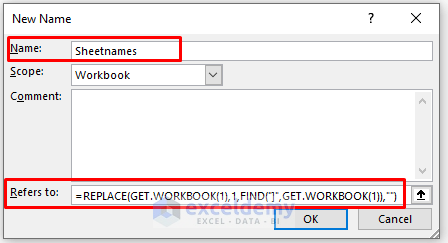
Step 2:
- Now, insert the formula with the the INDEX function where you want to get the list.
=INDEX(Sheetnames,C5)- Here, C5 is the starting cell of the serial number.

- Now link all the cells as mentioned in the previous method. Now click on any cells from the TOC and it will take you to the targeted worksheet.
- That’s how your TOC becomes fully functional.

Read More: How to Create Table of Contents in Excel with Hyperlinks
4. Use TRANSPOSE Function to Create Table of Contents in Excel
Furthermore, you can apply the TRANSPOSE function which returns a horizontal cell range as a vertical cell range, or vice versa. Let’s follow the instructions below to learn!
Steps:
- Before doing that make sure the Name is GetSheetName and insert the below formula.
=GET.WORKBOOK(1)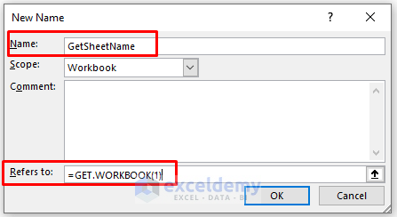
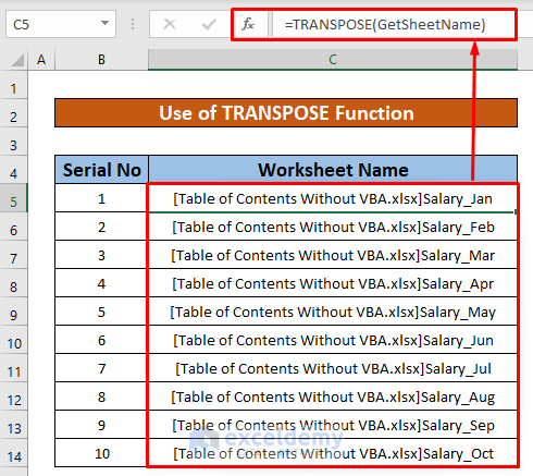
- Then insert the following formula in cell C5.
=TRANSPOSE(GetSheetName)
- Hence, simply ENTER on your keyboard. As a result, you will get the output of the TRANSPOSE function which has been given in the below screenshot.
Read More: How to Create Table of Contents in Excel with Page Numbers
5. Perform LOOKUP Function to Create Table of Contents in Excel
We can use the LOOKUP function to create a table of contents without VBA. Before using the LOOKUP function, create a new name where the Name may be Salary and the formula in the Refers to section. Let’s follow the instructions below to learn!
Steps:
- Before doing that make sure the Name is Salary and insert the below formula.
=GET.WORKBOOK(1)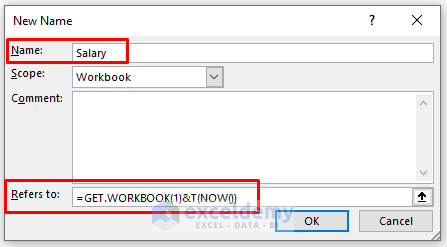
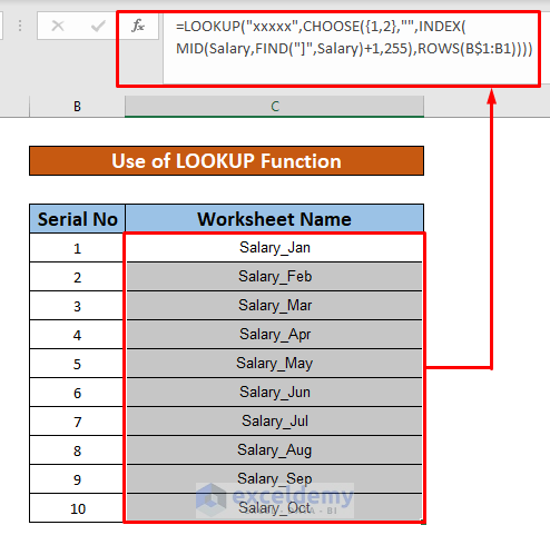
- Hence, write down the below formula in cell C5.
=LOOKUP("xxxxx",CHOOSE({1,2},"",INDEX(MID(Salary,FIND("]",Salary)+1,255),ROWS(B$1:B1))))- Further, ENTER on your keyboard. As a result, you will get Salary_Jan as the output of the LOOKUP function which has been given in the below screenshot.

- After that, AutoFill the LOOKUP function to the rest of the cells in column C.
Read More: How to Make Table of Contents Using VBA in Excel
6. Create Dynamic Table of Contents Using SUBSTITUTE Function
Moreover, you may create a dynamic table of contents using the SUBSTITUTE function. Let’s follow the instructions below to learn!
Step 1:
- Fix the name as Dynamic_Table_of_Contents and put the below formula.
=SUBSTITUTE(GET.WORKBOOK(1),"["&GET.WORKBOOK(16)&"]","")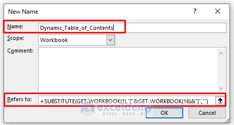
Step 2:
- Afterward, insert the following formula in cell C5.
=INDEX(Dynamic_Table_of_Contents,C5)- Further, ENTER on your keyboard. As a result, you will get the output of the dynamic function which has been given in the below screenshot.

Things to Remember
👉 #N/A! error arises when the formula or a function in the formula fails to find the referenced data.
👉 #DIV/0! error happens when a value is divided by zero(0) or the cell reference is blank.
Download Practice Workbook
Download this practice workbook to exercise while you are reading this article.
Conclusion
I hope all of the suitable steps mentioned above to create a table of contents without VBA will now provoke you to apply them in your Excel spreadsheets with more productivity. You are most welcome to feel free to comment if you have any questions or queries.
<< Go Back To Table of Contents in Excel | Hyperlink in Excel | Linking in Excel | Learn Excel
Get FREE Advanced Excel Exercises with Solutions!
