How to Create Table of Contents for Tabs in Excel (6 Methods)

Sometimes, the Excel workbook becomes large because of numerous worksheets. Because of having several worksheets, it is tough to overview all of them. In that case, a table of contents can be a good solution. This article will show how to create a table of contents for tabs using VBA code and hyperlinks in Excel. I think you find this article informative and get some valuable insides.

To create a table of contents for tabs, we have found six different ways through which you can easily do the work. In this article, we would like to utilize several Excel commands, functions, and more importantly, a VBA code to create a table of contents for tabs. Before doing anything, we need to create some spreadsheet tabs.

After that, we would like to utilize the Excel functions and VBA code to create the required table of contents for tabs.

1. Using Context Menu to Create Table of Contents for Tabs in Excel

Our first method is really easy to use. Here, we will write down each spreadsheet tab name and add a link there. Then, if we click on the link, it will take us to that certain worksheet. To understand the method, follow the steps.

Steps

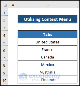
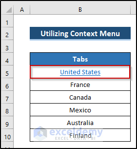
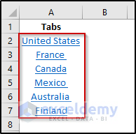
First, write down all the spreadsheet tabs where you want to add links.

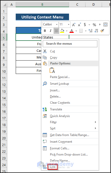
Then, right-click on cell B5.
It will open the Context Menu.
From there, select the Link option.

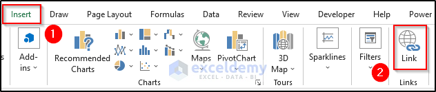
Another way you can get the Link option.
First, go to the Insert tab on the ribbon.
Then, select Link from the Links group.

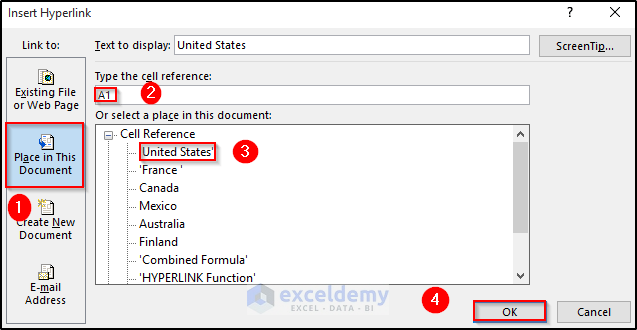
As a result, it will open the Insert Hyperlink dialog box.
Then, select Place in This Document from the Link to section.
After that, set any cell reference.
Then, select the place in this document. As we want to create a hyperlink of the United States worksheet, so, select the United States.
Finally, click on OK.

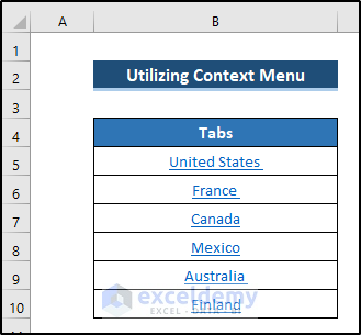
It will create a hyperlink on cell B5.

Follow the same procedure and add a hyperlink in every cell in your Table of Contents.

Then, if you click on any tabs, it will take us to that certain spreadsheet tab.

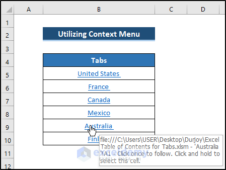
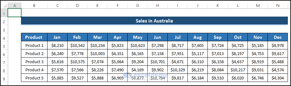
Here, we click on the Australia tab, and it takes us to the Australia spreadsheet tab. See the screenshot.

2. Applying Excel VBA Code to Create Table of Contents for Tabs

You can utilize VBA code to create a table of contents for tabs. Before doing anything, you need to add the Developer tab on the ribbon. After that, you use the VBA code and create a table of contents in Excel for tabs. Follow the steps.

Steps

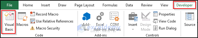
First, go to the Developer tab on the ribbon.
Then, select Visual Basic from the Code group.

It will open up the Visual Basic option.
Then, go to the Insert tab there.
After that, select the Module option.

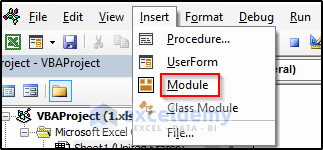
It will open a Module code window where you will write your VBA code.

Sub table_of_contents_for_tab()
 Dim xAlerts As Boolean
    Dim I  As Long
    Dim sheet_index As Worksheet
    Dim sheet_v As Variant
    xAlerts = Application.DisplayAlerts
    Application.DisplayAlerts = False
    On Error Resume Next
    Sheets("Table of contents").Delete
    On Error GoTo 0
    Set sheet_index = Sheets.Add(Sheets(1))
    sheet_index.Name = "Table of contents"
    I = 1
    Cells(1, 1).Value = "Tabs"
    For Each sheet_v In ThisWorkbook.Sheets
        If sheet_v.Name <> "Table of contents" Then
            I = I + 1
            sheet_index.Hyperlinks.Add Cells(I, 1), "", "'" & sheet_v.Name & "'!A1", , sheet_v.Name
        End If
    Next
    Application.DisplayAlerts = xAlerts
End Sub

Then, close the visual basic window.
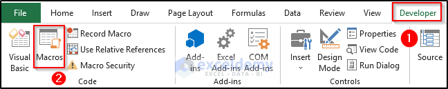
After that, go to the Developer tab again.
Select the Macros option from the Code group.

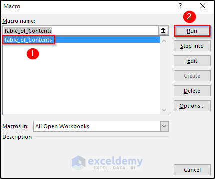
As a result, the Macro dialog box will appear.
Then, select the Table_of_Contents option from the Macro name section.
Finally, click on Run.

As a result, it will give us the following result. See the screenshot.

Then, if you select any tab, it will take it to that worksheet.

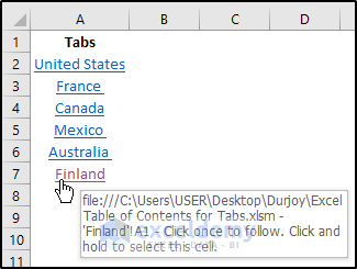
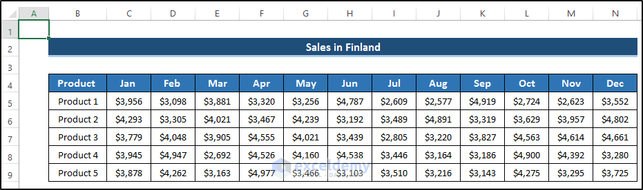
Here, we select the Finland tab, it will take us to the Finland spreadsheet tab. See the screenshot.

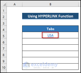
3. Using HYPERLINK Function

In this method, we will utilize the HYPERLINK function. By using the HYPERLINK function, we create a table of contents for tabs. After that, if you click on the tab, it will take you to that certain spreadsheet tab. To understand this method, follow the steps carefully.

Steps

First, select cell B5.
Then, write down the following formula.

=HYPERLINK("#'United States'!A1","USA")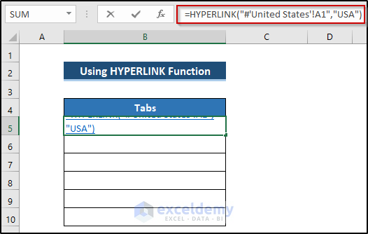

After that, press Enter to apply the formula.

Then, select cell B6.
Write down the following formula.

=HYPERLINK("#'France '!A1","France")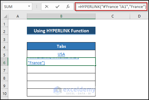

Then, press Enter to apply the formula.

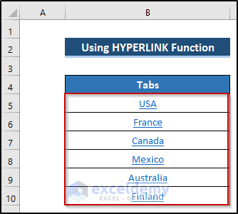
Do the same procedure for other cells to create a table of contents for tabs.
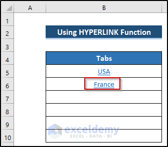
Finally, we will get the following result.

Then, if you select any tab, it will take it to that spreadsheet tab.

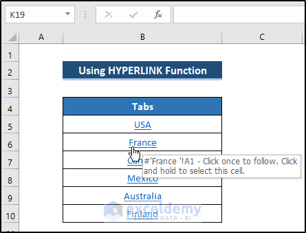
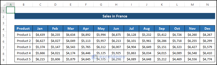
Here, we select the France tab, it will take us to the France spreadsheet tab. See the screenshot.

4. Use of Power Query to Create Table of Contents for Tabs in Excel

Our fourth method is based on using the power query. First of all, we open the Excel file on the power query. Then, using the HYPERLINK function, we will get the hyperlinks for each worksheet. To understand this properly, follow the steps.

Steps

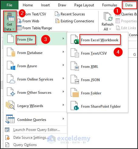
First, go to the Data tab on the ribbon.
Then, select Get Data drop-down option from the Get & Transform Data.
After that, select From File option.
Then, select From Excel Workbook.

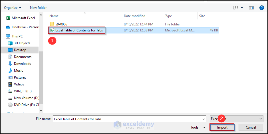
After that, select your preferred Excel file and click on Import.

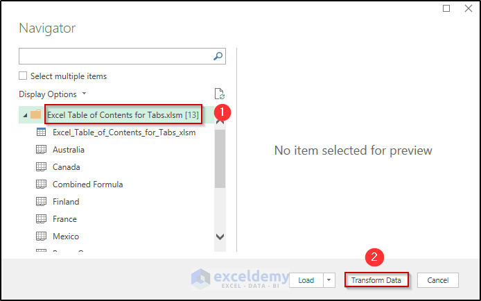
Then, the Navigator dialog box will appear.
Select the Table of Contents option.
Finally, click on Transform Data.

As a result, it will open up the Power Query window.

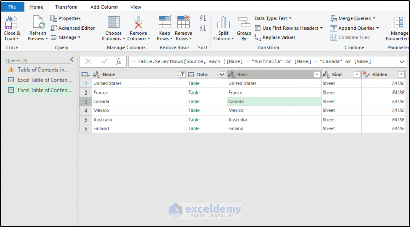
Then, right-click on the Name title and select Remove Other Columns.

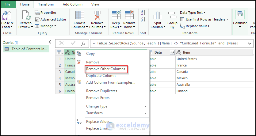
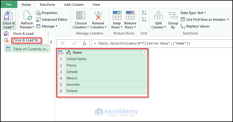
As a result, all other columns are removed.
Then, click on the Close & Load drop-down option.
From there, select Close & Load To.

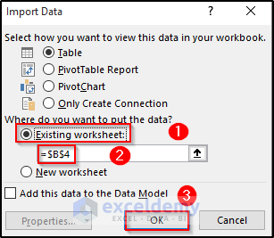
Then, the Import Data dialog box will appear.
Select the place where you want to put your data and also set the cell.
Finally, click on OK.

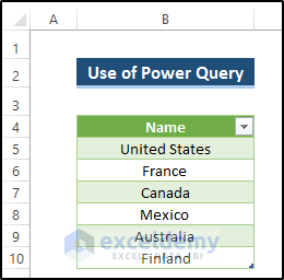
It will give us the following result. See the screenshot.

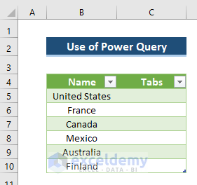
Then, create a new column where you want to put your tabs link.

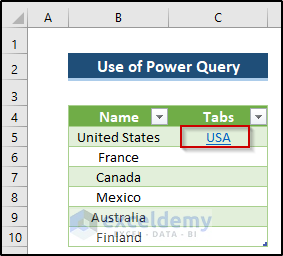
After that, select cell C5.
Write down the following formula.

=HYPERLINK("#'"&[@Name]&"'!A1","USA")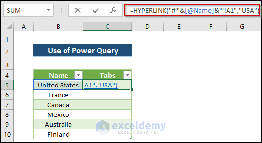

Press Enter to apply the formula.

Do the same procedure for all cells. After that, you will get the following result.

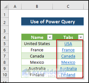
If you click on any tab, it will take you to that certain worksheet.
Here, we click on the USA tab. It takes us to the United States spreadsheet tab.

5. Use of Buttons to Create Table of Contents for Tabs

Another way we can create a table of contents for tabs is by using the Buttons. In this method, we create a button and then link it to the desired spreadsheet tab. After that, if we click on the button, it will take us to that tab. To understand the method, follow the steps properly.

Steps

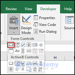
First, go to the Developer tab on the ribbon.
Then, select the Insert drop-down option from the Controls group.

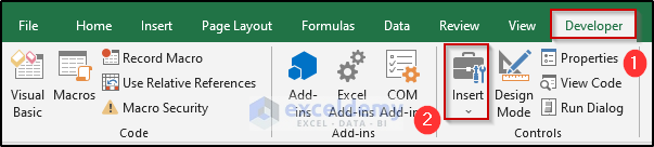
Select the Button(Form Control) from the Insert drop-down option.

As a result, it will convert the mouse cursor into a plus (+) icon.
Drag the plus icon to give the shape of the button.

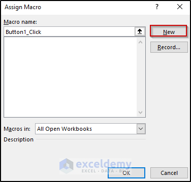
It will open the Assign Macro dialog box.
Then, select the New option.

It will open the Visual Basic window where you need to put your VBA for this button.
This code will create a link to a certain spreadsheet tab.
Write down the following code.

Sub Button1_Click()
ThisWorkbook.Sheets("United States").Activate
End Sub

Note: To create a link to a certain spreadsheet tab, you need to replace ‘United States’ with your preferred tab name. All other codes will remain unchanged.

Then, close the window.
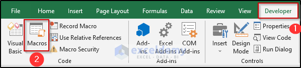
After that, go to the Developer tab on the ribbon.
Then, select Macros from the Code group.

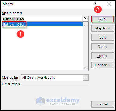
As a result, the Macro dialog box will appear.
Then, select Button1_Click from the Macro name section.
Finally, click on Run.

It will take us to that certain tab.
Then, right-click on the button.
Select Edit Text from the Context Menu.

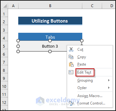
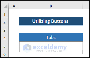
Here, we set our button name as ‘USA’.
You can set your preferred name.
Now, click on the Name of the button.
It will take you to that certain tab.

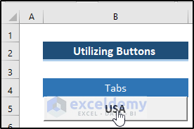
Here, we create a link with the spreadsheet tab named ‘United States’. So, it will take us to that tab.

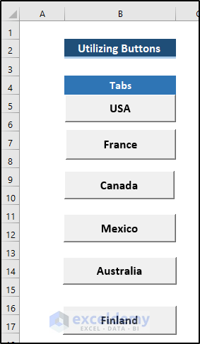
Follow the same procedure to create other buttons for all required tabs.
Finally, we get the required table of contents for tabs. See the screenshot.

6. Applying Combined Formula to Create Table of Contents

In this method, we utilize the Name Manager where we will define the name. After that, we will use a combined formula through which we can create the table of contents for tabs. Before we get into the steps, here are the functions we are going to use in this method:

To understand the method clearly, now follow the steps.

Steps

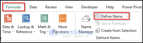
First, go to the Formula tab in the ribbon.
Then, select Define Name from the Defined Names group.

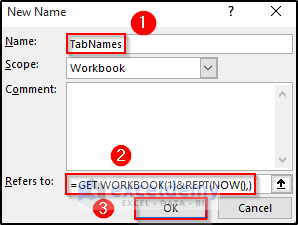
It will open the New Name dialog box.
Then, in the Name section, put TabNames as the name.
After that, write down the following formula in the Refers to section.

=GET.WORKBOOK(1)&REPT(NOW(),)

Finally, click on OK.

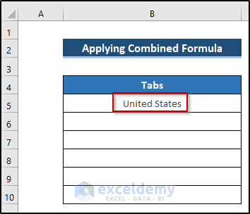
Then, select cell B5.
Write down the following formula using the combined formula.

=IF(ROW(A1)>SHEETS(),REPT(NOW(),),SUBSTITUTE(HYPERLINK("#'"&TRIM(RIGHT(SUBSTITUTE(SUBSTITUTE(INDEX(TabNames,ROW(A1))," ",CHAR(255)),"]",REPT(" ",32)),32))&"'!A1",TRIM(RIGHT(SUBSTITUTE(SUBSTITUTE(INDEX(TabNames,ROW(A1))," ",CHAR(255)),"]",REPT(" ",32)),32))),CHAR(255)," "))

This formula was taken from Professor-Excel which helped us to give the following output.

Then, press Enter to apply the formula.

After that, drag the Fill Handle icon down the column.

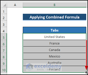
Then, if you click on any tab, it will take you to that spreadsheet tab.

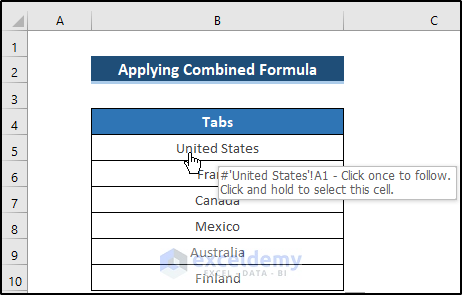
Here, we click on the United States tab, and it takes us to the United States spreadsheet tab. See the screenshot.

Download Practice Workbook

Download the practice workbook below.

Table of Contents for Tabs.xlsm

Conclusion

To create an Excel table of contents for tabs, we have shown six different methods through which you can create a better version of it. To create this, we utilize several Excel functions and VBA code. All of these methods are fairly effective and user-friendly. In this article, we have shown how to utilize buttons to create a table of contents. I think we covered all possible areas regarding the table of contents. If you have further questions, feel free to ask in the comment box.

<< Go Back To Table of Contents in Excel | Hyperlink in Excel | Linking in Excel | Learn Excel

Get FREE Advanced Excel Exercises with Solutions!

How to Create Table of Contents for Tabs in Excel (6 Methods)

1. Using Context Menu to Create Table of Contents for Tabs in Excel

2. Applying Excel VBA Code to Create Table of Contents for Tabs

3. Using HYPERLINK Function

4. Use of Power Query to Create Table of Contents for Tabs in Excel

5. Use of Buttons to Create Table of Contents for Tabs

6. Applying Combined Formula to Create Table of Contents

Conclusion

Leave a reply Cancel reply