Method 1 – Utilizing Keyboard Shortcut to Create Table of Contents
Steps:
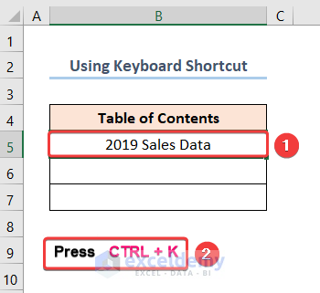
- Type in the name of the worksheet. In this case, the name of our worksheet is 2019 Sales Data.
- Press the CTRL + K key on your keyboard.
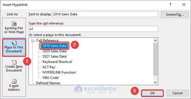
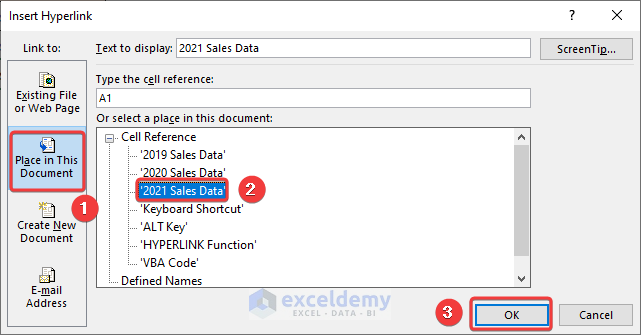
This brings up the Insert Hyperlink wizard.
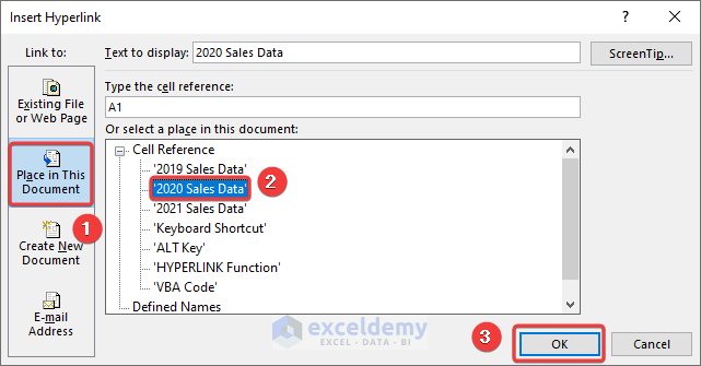
- Click the Place in This Document option >> then choose the worksheet name (2019 Sales Data) >> click the OK button.
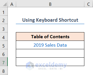
This inserts a clickable link into the text string as shown in the image below.
Repeat the process for the 2020 Sales Data worksheet.
Follow the same procedure for the 2021 Sales Data worksheet.
The results should look like the picture given below.
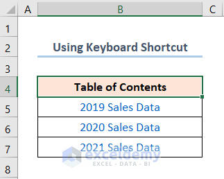
You generated a table of contents for your worksheets.
Method 2 – Employing ALT Key to Generate Table of Contents
Steps:
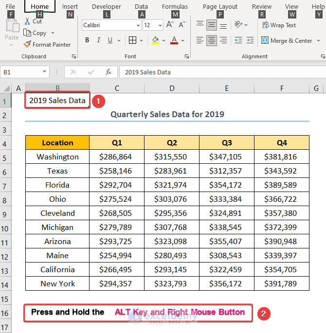
- Select the heading (here it is 2019 Sales Data).
- Press and hold down the ALT Key and the right mouse button.
Note: This method will only work if your worksheet has been saved. Press the CTRL + S key to save your worksheet first.
- Hover the cursor at the edge of the selected B1 cell and drag it into the worksheet with the table of contents. It is the ALT Key worksheet.
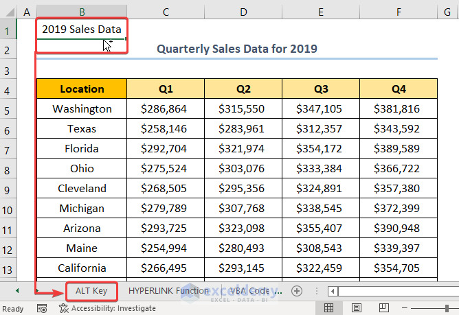
This brings you to the ALT Key worksheet.
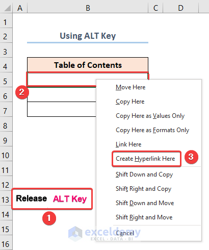
- Release the ALT key and drag the cursor to the desired location (B5 cell) while holding the right mouse button.
- Let go of the right mouse button >> a list of options appears; choose the Create Hyperlink Here option.
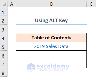
The results should look like the following image below.
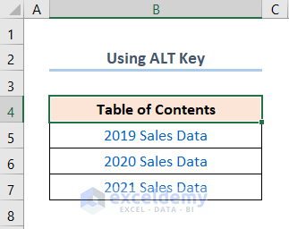
Repeat the same procedure for the other two worksheets as depicted below.
Method 3 – Using HYPERLINK Function to Create Table of Contents
Steps:
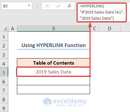
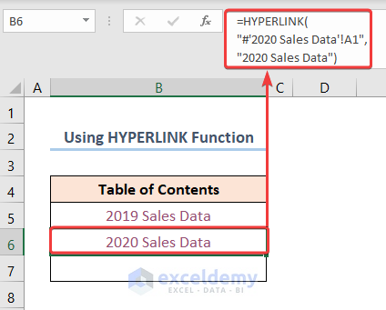
- Go to the B5 cell and enter the expression below.
=HYPERLINK("#'2019 Sales Data'!A1","2019 Sales Data")
The “#’2019 Sales Data’!A1” is the link_location argument and refers to the location of the 2019 Sales Data worksheet. The “2019 Sales Data” is the optional friendly_name argument, which indicates the text string displayed as the link. The Pound (#) sign tells the function that the worksheet is in the same workbook.
- Follow the same process for the 2020 Sales Data worksheet and insert the formula given below.
=HYPERLINK("#'2020 Sales Data'!A1","2020 Sales Data")
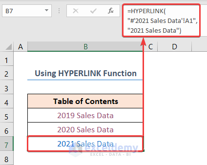
- Type in the expression below to repeat the 2021 Sales Data worksheet procedure.
=HYPERLINK("#'2021 Sales Data'!A1","2021 Sales Data")
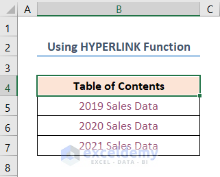
After completing all the steps, the results should look like the image below.
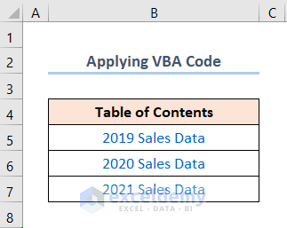
Method 4 – Applying VBA Code to Create Automatic Table of Contents
Step 1: Open Visual Basic Editor
- Navigate to the Developer tab >> click the Visual Basic button.
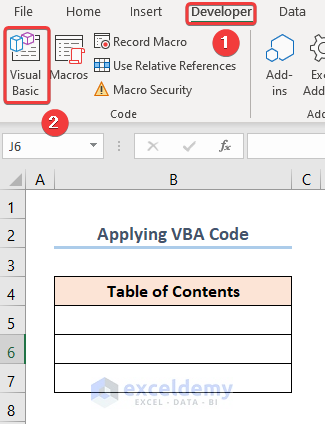
This opens the Visual Basic Editor in a new window.
Step 2: Insert VBA Code
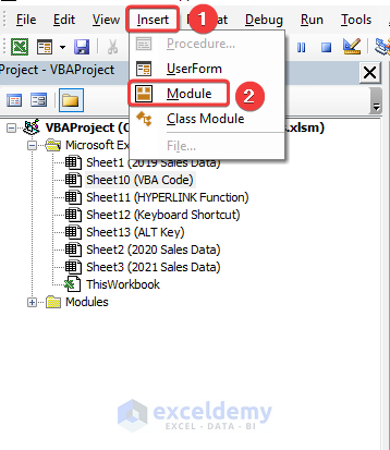
- Go to the Insert tab >> Select Module.
Copy the code from here and paste it into the window below.
Sub Excel_Table_Of_Contents()

    Dim alerts As Boolean
    Dim y  As Long
    Dim Wrksht_Index As Worksheet
    Dim Wrksht As Variant

    alerts = Application.DisplayAlerts
    Application.DisplayAlerts = False
    On Error Resume Next
    Sheets("TOC").Delete
    On Error GoTo 0
    Set Wrksht_Index = Sheets.Add(Sheets(1))
    Wrksht_Index.Name = "TOC"
    y = 1
    Cells(1, 1).Value = "TOC"
    For Each Wrksht In ThisWorkbook.Sheets
        If Wrksht.Name <> "TOC" Then
            y = y + 1
            Wrksht_Index.Hyperlinks.Add Cells(y, 1), "", "'" & Wrksht.Name & "'!A1", , Wrksht.Name
        End If
    Next
    Application.DisplayAlerts = alerts
End Sub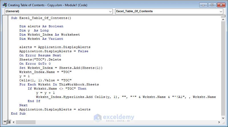
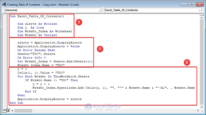
⚡ Code Breakdown:
The VBA code is used to generate the table of contents. The code is divided into 3 steps.
- The sub-routine is given a name; it is Excel_Table_Of_Contents().
- Define the variables alerts, y, and Wrksht.
- Assign Long, Boolean, and Variant data types.
- Define Wrksht_Index as the variable for storing the Worksheet object.
- Remove any previous Table of Contents sheet using the Delete method.
- Insert a new sheet with the Add method in the first position and name it “Table of contents” using the Name statement.
- We declare a counter (y = 1) and use the For Loop and the If statement to obtain the names of the worksheets.
- Use the HYPERLINK function to generate clickable links embedded in the worksheet names.
Step 3: Running VBA Code
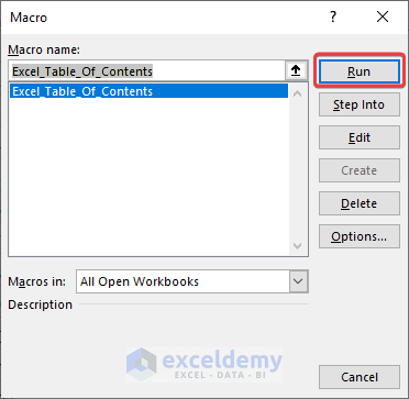
- Press the F5 key on your keyboard.
This opens the Macros dialog box.
- Click the Run button.
The results should look like the screenshot given below.
Navigating to Worksheets Using Status Bar
Steps:
- Move your cursor to the bottom-left corner of your worksheet, as shown in the picture below.
- Hover the cursor, and you’ll see a Right click to See all sheets message.
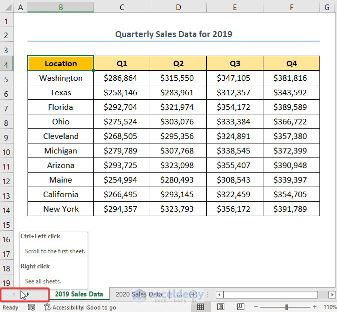
- Right-click with the mouse.
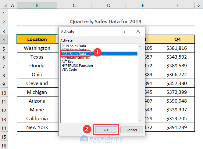
The Activate dialog box pops up, which displays all the sheets.
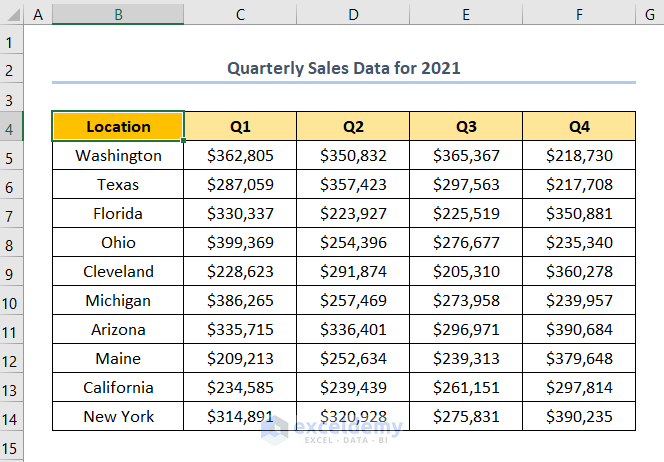
- Choose the sheet; we’ve chosen the 2021 Sales Data >> click OK.
Move to the sheet that you’ve chosen.
Download Practice Workbook
You can download the practice workbook from the link below.
Related Articles
- How to Create Table of Contents in Excel with Page Numbers
- How to Create Table of Contents for Tabs in Excel
<< Go Back To Table of Contents in Excel | Hyperlink in Excel | Linking in Excel | Learn Excel
Get FREE Advanced Excel Exercises with Solutions!

I created a Table of Contents with the sheet names but under the sheet names, I want a list of titles on the linked sheet that I can click to go directly to that spot on the sheet. I know I can do this manually, but I want to set it up so that if I insert or delete rows, the links will update to the new location. I hope that makes sense.
Hello Julie Parker,
Thank you for your question. I have looked into this matter, and so far, I haven’t been able to find a solution to your particular query. In the meantime, I have prepared an excel template with a table of contents that you may download from the link below. That said, I will let you know when I find a solution. I hope this was helpful.
Table of Contents.xlsx