Method 1 – Use Link to Create Table of Contents with Page Numbers
Step 1: Insert Page Numbers in Individual Worksheets
Insert page numbers in the worksheets.
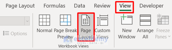
- Go to the View tab and select Page Layout from the Workbook Views group.
- You will notice 3 blocks in the upper Header section on the page.
- Similar blocks will also appear in the Footer section below.
- Click on any block where you want the page number.

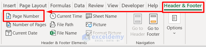
- Go to the Header & Footer tab.
- Select Page Number under the Header & Footer Elements group.
- You will see the &[Page] appear on the Header block.
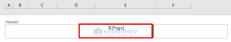
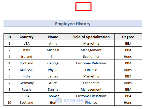
- Click any cell of the worksheet and you will see the page number.
- In addition to that, type ‘of’ after &[Page] and then go to the Header & Footer tab.
- Select the Number of Pages option.
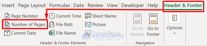
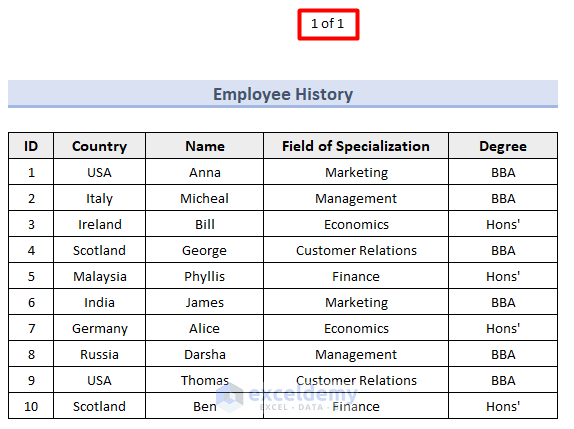
- The Header block will look like this:

- Click any cell to show the page number among all the pages.
- Apply the same procedure for other worksheets as well.
Step 2: Create Table of Contents with Link
- Create a new worksheet where you want to create the table of contents.
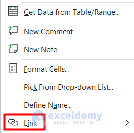
- In this worksheet, right-click on cell B4.
- Select Link from its Context Menu.
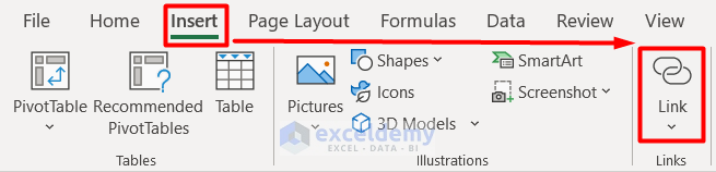
- You will get this Link command under the Insert tab.
- The Insert Hyperlink window pops up.
- Select Place in this Document.
- Choose the first worksheet Employee History.
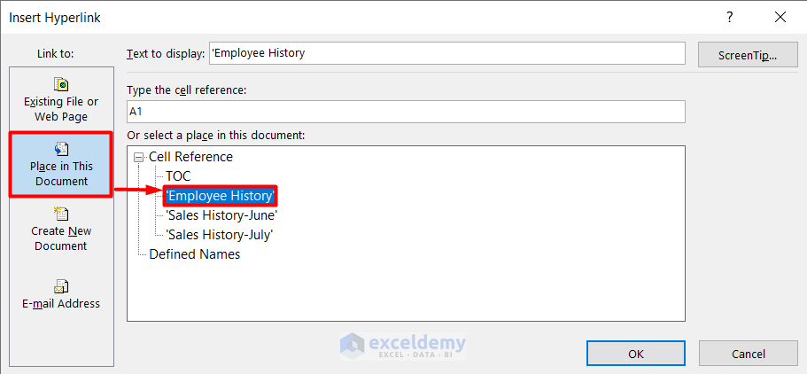
- Insert the page number beside the worksheet name in the Text to display box.
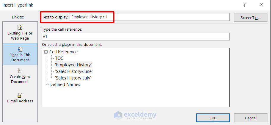
- Press OK.
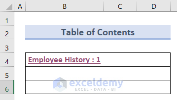
- You will see that the worksheet is inserted as a table of contents.
- Follow the similar procedure for other worksheets as well.
- After some formatting in cells, you will get the final result like this:
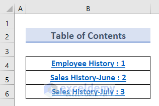
- Click on any of the worksheet names, and it will direct you to that page.
Method 2 – Make Table of Contents Using Excel GET.WORKBOOK Function
- You need to name the worksheets along with the page numbers, like the following image.

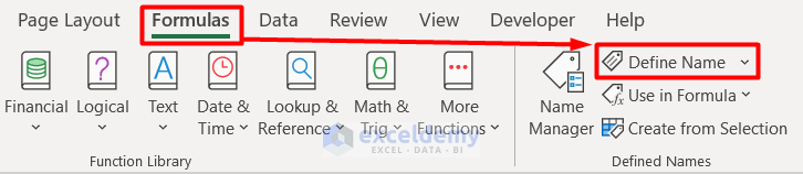
- Open a new sheet, “TOC,” where you want to create a table of contents with page numbers and go to the Formulas tab.
- Select Define Name under the Define Names group.
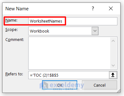
- A New Name window appears.
- Type WorksheetNames in the Name box.
- Type this formula in the Refers to box.
=GET.WORKBOOK(1)&REPT(NOW(),)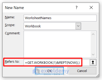
- After that, press OK.
- Select the cell where you want to insert the name of the first worksheet. We selected cell B4.
- Insert this formula in cell B4.
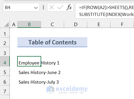
=IF(ROW(A2)>SHEETS(),REPT(NOW(),),SUBSTITUTE(HYPERLINK("#'"&TRIM(RIGHT(SUBSTITUTE(SUBSTITUTE(INDEX(WorksheetNames,ROW(A2))," ",CHAR(255)),"]",REPT(" ",32)),32))&"'!A1",TRIM(RIGHT(SUBSTITUTE(SUBSTITUTE(INDEX(WorksheetNames,ROW(A2))," ",CHAR(255)),"]",REPT(" ",32)),32))),CHAR(255)," "))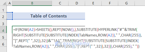
- Press Enter.
- It will show the 1st worksheet name in your workbook.
- Apply the same formula for cells B5 and B6 where the ROW in the formula will be A3 and A4 respectively.
- The final output looks like this:
Method 3 – Apply Excel VBA Macro to Make Table of Contents with Page Numbers
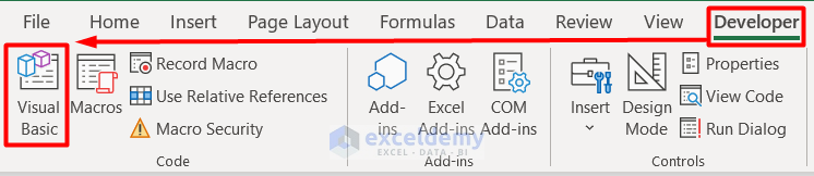
- Go to the Developer tab.
- Select Visual Basic under the Code group.
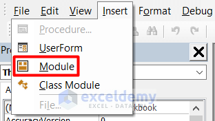
- Following the Visual Basic window, select Module from the Insert section.
- Insert this code on the blank page and click on the Run Sub button or press F5 on your keyboard.
Sub CreateTableofcontents()
    Dim yAlerts As Boolean
    Dim L As Long
    Dim xSheetIndex As Worksheet
    Dim xSt As Variant
    yAlerts = Application.DisplayAlerts
    Application.DisplayAlerts = False
    On Error Resume Next
    Sheets("Table of contents").Delete
    On Error GoTo 0
    Set xSheetIndex = Sheets.Add(Sheets(1))
    xSheetIndex.Name = "Table of contents"
    L = 2
    Cells(2, 2).Value = "Table of contents"
    For Each xSt In ThisWorkbook.Sheets
        If xSt.Name <> "Table of contents" Then
           L = L + 2
            xSheetIndex.Hyperlinks.Add Cells(L, 2), "", "'" & xSt.Name & "'!A1", , xSt.Name
        End If
    Next
    Application.DisplayAlerts = yAlerts
End Sub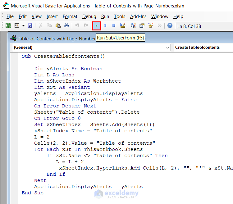
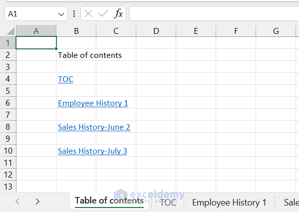
- You will get the table of contents based on the worksheets on a new sheet.
Download Workbook
Download the sample file from here to practice by yourself.
Related Articles
- How to Create Table of Contents Automatically in Excel
- How to Create Table of Contents for Tabs in Excel
<< Go Back To Table of Contents in Excel | Hyperlink in Excel | Linking in Excel | Learn Excel
Get FREE Advanced Excel Exercises with Solutions!

I get a “Name? errror
Hello,
Thanks for your comment.
There was a small mistake in the formula. That’s why it is giving a Name error. The article and workbook are corrected and updated accordingly. If you have other queries let us know in the comment.
Regards,
Sajid Ahmed
Exceldemy
For #block error, you will need to go to options<trust center<trust center settings<click on enable excel 4.0. Click ok then close your file then reopen. It should work. Remember to close out because I update the file but didn't close and restart it didn't work initially. Hopefully that helps.
Hello Jason Ngo,
Thanks for your suggestion, we appreciate it deeply.Enabling Excel 4.0 macros and restarting the file should indeed help with resolving the #block error. Your step-by-step explanation is really helpful, especially the reminder to close and reopen the file for the changes to take effect. Much appreciated.
Regards
ExcelDemy