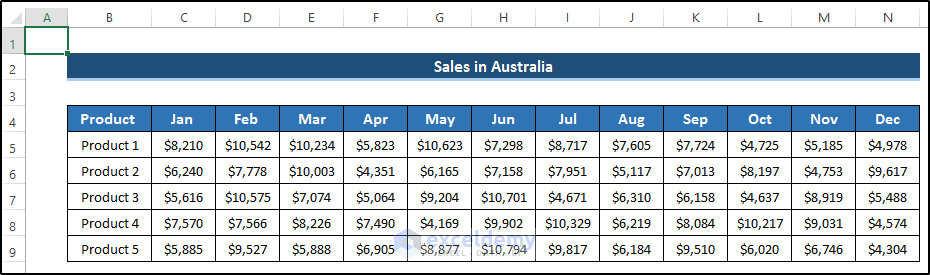
Sometimes, the Excel workbook becomes large because of numerous worksheets. Because of having several worksheets, it is tough to overview all of them. In that case, a table of contents can be a good solution. This article will show how to create a table of contents in Excel with hyperlinks. Basically, using hyperlinks in a table of contents can make it dynamic. I hope you find this article very interesting and gain lots of knowledge regarding the topic.
How to Create Table of Contents in Excel with Hyperlinks: 5 Easy Methods
To create a table of contents in Excel with hyperlinks, we have found five different methods through which you can solve the problem quite easily. In this article, we would like to utilize several Excel commands, functions, and more importantly, a VBA code to create a table of contents in Excel with hyperlinks.
1. Utilizing Context Menu
Our Initial method is really easy to use. Here, we will write down each worksheet’s name and provide a link there. Then, if we click on the link, it will take us to that certain worksheet. To understand the method, follow the steps.
Steps
- First, write down all the names where you would like to add links.

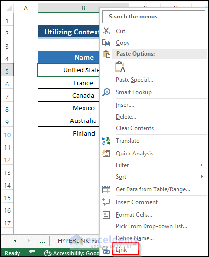
- Then, right-click on cell C5.
- It will open the Context Menu.
- From there, select the Link option.
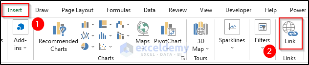
- Another way you can get the Link option
- First, go to the Insert tab on the ribbon.
- Then, select Link from the Links group.
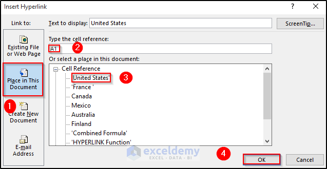
- As a result, it will open the Insert Hyperlink dialog box.
- Then, select Place in This Document from the Link to section.
- After that, set any cell reference.
- Then, select the place in this document. As we want to provide a hyperlink to the United States worksheet, so, select the United States.
- Finally, click on OK.
- It will create the hyperlink on cell C5.

- Follow the same procedure and add a hyperlink in every cell in the Table of Contents.
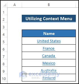
- Then, if you click on any link, it will take you to that certain worksheet.

- Here, we click on the Australia hyperlink, and it takes us to the Australia worksheet. See the screenshot.
Read More: How to Create Table of Contents Automatically in Excel
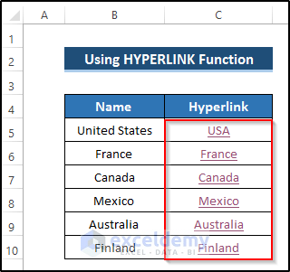
2. Using HYPERLINK Function
In this method, we will utilize the HYPERLINK function. By using the HYPERLINK function, we create a link with a certain worksheet. After that, if you click on the link, it will take you to that certain worksheet. To understand this method, follow the steps carefully.
Steps
- First, select cell C5.
- Then, write down the following formula.
=HYPERLINK("#'United States'!A1","USA")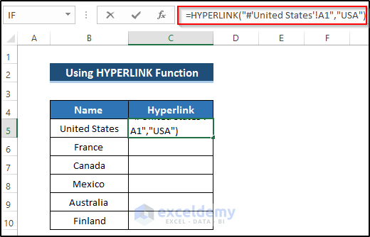
- After that, press Enter to apply the formula.
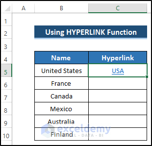
- Then, select cell C6.
- Write down the following formula.
=HYPERLINK("#'France '!A1","France")
- Then, press Enter to apply the formula.
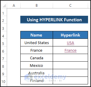
- Do the same procedure for other cells to create a hyperlink for every worksheet.
- Finally, we will get the following result.
- Then, if you select any hyperlink, it will take it to that worksheet.

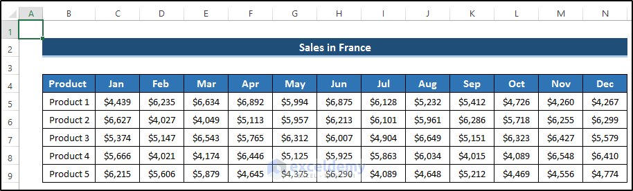
- Here, we select the France hyperlink, it will take us to the France worksheet. See the screenshot.
Read More: How to Create Table of Contents in Excel with Page Numbers
3. Embedding VBA Code
You can utilize VBA code to create a table of content with hyperlinks. Before doing anything, you need to add the Developer tab on the ribbon. After that, you use the VBA code and create a table of content in Excel with hyperlinks. Follow the steps.
Steps
- First, go to the Developer tab on the ribbon.
- Then, select Visual Basic from the Code group.

- It will open up the Visual Basic window.
- Then, go to the Insert tab there.
- After that, select the Module option.

- It will open a Module code window where you will write your VBA code.
- Write down the following code.
Sub Table_of_Contents()
    Dim worksheet_value As Worksheet
    Dim worksheet_name, Link_sheet, output_sheet_name As String
    Dim j As Integer
    Sheets.Add
    output_sheet_name = "Table of Contents"
    ActiveSheet.Name = output_sheet_name
    Range("B3") = output_sheet_name
    j = 0
    For Each worksheet_value In Worksheets
            worksheet_name = worksheet_value.Name
            Link_sheet = "'" & worksheet_name & "'!R1C1"
            Sheets(output_sheet_name).Cells(j + 5, 2) = worksheet_name
            Sheets(output_sheet_name).Cells(j + 5, 2).Select
            ActiveSheet.Hyperlinks.Add Anchor:=Selection, Address:="", SubAddress:=Link_sheet
            j = j + 1
    Next
End Sub- Then, close the visual basic window.
- After that, go to the Developer tab again.
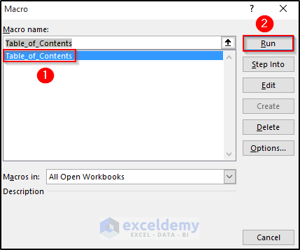
- Select the Macros option from the Code group.

- As a result, the Macro dialog box will appear.
- Then, select the Table_of_Contents option from the Macro name section.
- Finally, click on Run.
- As a result, it will give us the following result. See the screenshot.
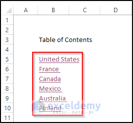
- Then, if you select any hyperlink, it will take it to that worksheet.

- Here, we select the Finland hyperlink, it will take us to the Finland worksheet. See the screenshot.

Read More: How to Make Table of Contents Using VBA in Excel
4. Use of Power Query
Our third method is based on using the power query. First of all, we open the Excel file on the power query. Then, using the HYPERLINK function, we will get the hyperlinks for each worksheet. To understand this properly, follow the steps.
Steps
- First, go to the Data tab on the ribbon.
- Then, select Get Data drop-down option from the Get & Transform Data group.
- After that, select From File option.
- Then, select From Excel Workbook.

- After that, select your preferred Excel file and click on Import.

- Then, the Navigator dialog box will appear.
- Select the Table of Contents.
- Finally, click on Transform Data.

- As a result, it will open up the Power Query window.
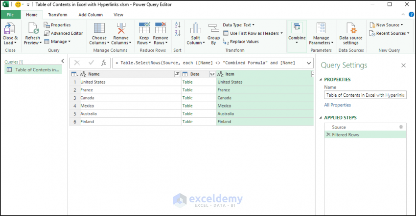
- Then, right-click on the Name title and select Remove Other Columns.

- As a result, all other columns are removed.
- Then, click on the Close & Load drop-down option.
- From there, select Close & Load To.

- Then, the Import Data dialog box will appear.
- Select the place where you would like to put your data and also set the cell.
- Finally, click on OK.

- It will give us the following result. See the screenshot.
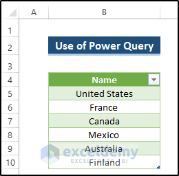
- Then, create a new column where you would like to put your hyperlinks.

- After that, select cell C5.
- Write down the following formula.
=HYPERLINK("#'"&[@Name]&"'!A1","USA")
- Press Enter to apply the formula.

- Do the same procedure for all cells. After that, you will get the following result.

- If you click on any name, it will take you to that certain worksheet.
- Here, we click on the USA hyperlink. It takes us to the United States worksheet.

Read More: How to Create Table of Contents Without VBA in Excel
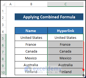
5. Applying Combined Formula
In this method, we utilize the Name Manager where we will define the name. After that, we will use a combined formula through which we can create the table of contents with hyperlinks. Before we get into the steps, here are the functions we are going to use in this method:
- REPT Function
- NOW Function
- SHEETS Function
- ROW Function
- SUBSTITUTE Function
- HYPERLINK Function
- TRIM Function
- RIGHT Function
- CHAR Function
To understand the method clearly, now follow the steps.
Steps
- First, go to the Formula tab in the ribbon.
- Then, select Define Name from the Defined Names group.

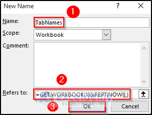
- It will open the New Name dialog box.
- Then, in the Name section, put TabNames as the name.
- After that, write down the following formula in the Refers to section:
=GET.WORKBOOK(1)&REPT(NOW(),)- Finally, click on OK.
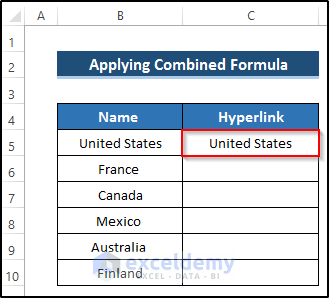
- Then, select cell C5.
- Write down the following formula using the combined formula.
=IF(ROW(A1)>SHEETS(),REPT(NOW(),),SUBSTITUTE(HYPERLINK("#'"&TRIM(RIGHT(SUBSTITUTE(SUBSTITUTE(INDEX(TabNames,ROW(A1))," ",CHAR(255)),"]",REPT(" ",32)),32))&"'!A1",TRIM(RIGHT(SUBSTITUTE(SUBSTITUTE(INDEX(TabNames,ROW(A1))," ",CHAR(255)),"]",REPT(" ",32)),32))),CHAR(255)," "))This formula was taken from Professor-Excel which helped us to give the following output.
- Then, press Enter to apply the formula.
- After that, drag the Fill Handle icon down the column.
- Then, if you click on the hyperlink option, it will take you to that worksheet.

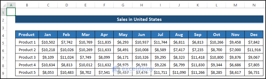
- Here, we click on the United States hyperlink, and it takes us to the United States worksheet. See the screenshot.
Read More: How to Create Table of Contents for Tabs in Excel
Download Practice Workbook
Download the practice workbook below.
Conclusion
We have shown five different methods to create a table of contents in Excel with hyperlinks. In this article, we will try to focus on how to include hyperlinks in the table content so that you can easily access each worksheet. To do this, we used several Excel functions and VBA code. All of these are fairly easy to understand. If you have any questions, feel free to ask in the comment box.
<< Go Back To Table of Contents in Excel | Hyperlink in Excel | Linking in Excel | Learn Excel
Get FREE Advanced Excel Exercises with Solutions!
