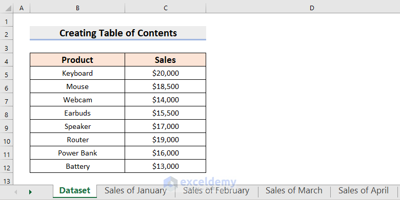
We will use a sample dataset, which has 2 Columns, Product and Sales, across 5 worksheets, Dataset, Sales of January, Sales of February, Sales of March, and Sales of April.
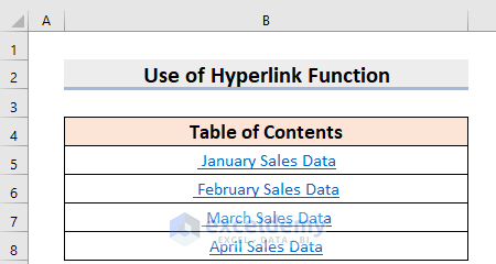
Method 1 – Using HYPERLINK Function to Create a Table of Contents in Excel
The HYPERLINK function to create a Table of Contents in Excel. The steps are given below.
Steps:
- Select a different cell (such as B5) where you want to see the contents. The best option is to create the Table of Contents in a new worksheet.
- Enter this formula in the cell.
=HYPERLINK("#'Sales of January'!A1"," January Sales Data")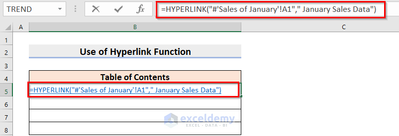
Formula Breakdown
- The HYPERLINK function will create a link to go to a particular worksheet.
- Sales of January is the name of the worksheet for which I want to create a link.
- Hash Tag (#) will find the worksheet.
- Exclamatory (!) A1 represents the Cell Location of the Sheet named Sales of January.
- January Sales Data is the Friendly Name which means this name will be in the Content name.
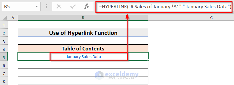
- Press Enter to get the result.
- Repeat the procedure again for the sheet named Sales of February.
- Use the corresponding formula in the B6:
=HYPERLINK("#'Sales of February'!A1"," February Sales Data")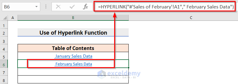
- In the same way, you have to write the formula individually in the cells.
Read More: How to Create Table of Contents in Excel with Hyperlinks (5 Ways)
Method 2 – Applying Excel Power Query for Creating a Table of Contents
Steps:
- Go to the worksheet where you want to create a Table of Contents.
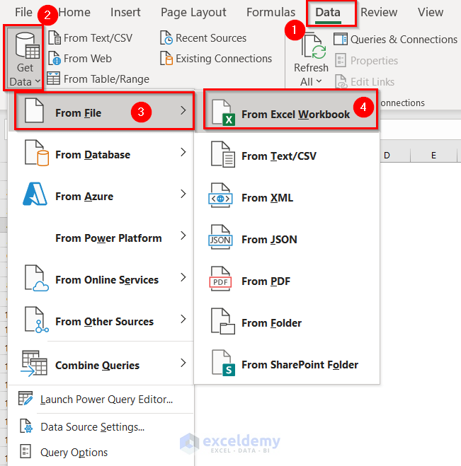
- From the Data tab, choose Get Data.
- Select From File and choose From Excel Workbook
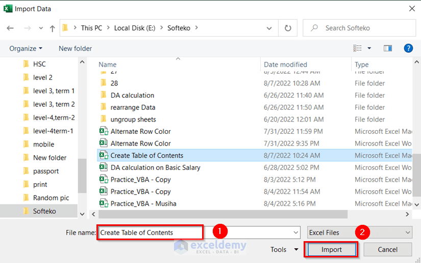
A window named Import Data will appear.
- Choose your Excel file. We have chosen Create Table of Contents.
- Press Import.
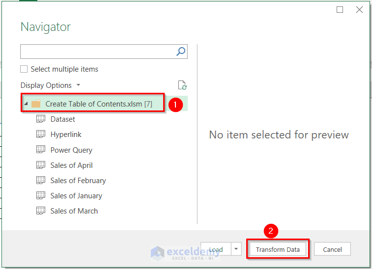
A dialog box named Navigator will appear.
- Select your Excel file from the dialog box.
- Click on Transform Data. Here, if you don’t select the Excel file, you will not be able to click on the Transform Data.
You will see the following Power Query Editor window.
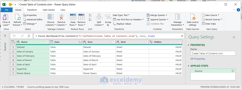
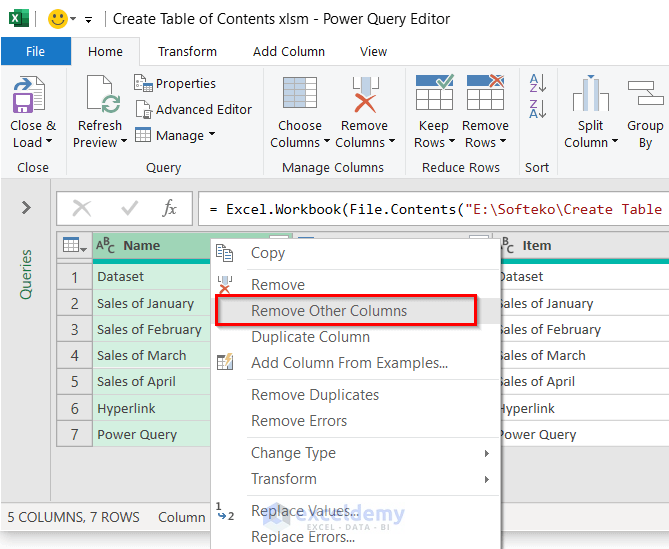
- Right-click on the Name column.
- From the Context Menu Bar, select Remove Other Columns.
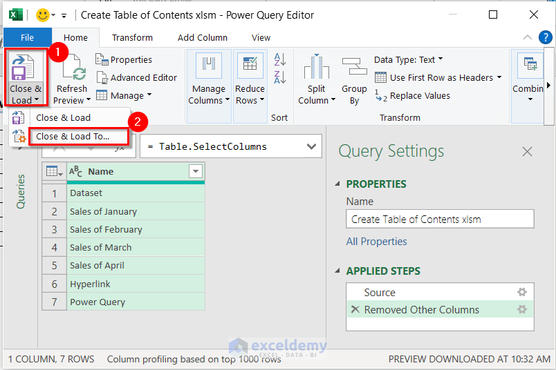
- From Close & Load, select Close & Load To…
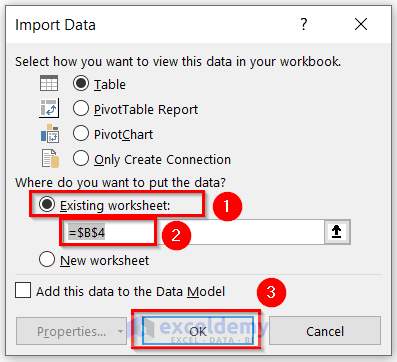
A dialog box named Import Data will appear.
- Select the Existing worksheet. Here, you can choose a New worksheet also. In that case, your Table of Contents will be in a different and new worksheet.
- Choose the Cell location for the Table of Contents. We have chosen B4 as my Cell location.
- Press OK.
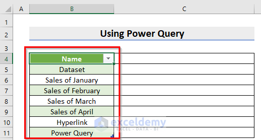
You will see the following Contents.
To create the link, follow the procedure given below.
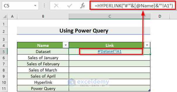
- Select a different cell C5 where you want to see the contents.
- Use this formula in C5:
=HYPERLINK("#'"&[@Name]&"'!A1")Here, we selected the name of the worksheet from cell B5 (Dataset).
Formula Breakdown
- The HYPERLINK function will create a link to go to a particular worksheet.
- Hash Tag (#) will ensure that the worksheet is in the same workbook.
- @Name denotes the name of the worksheet for which you want to create the link.
- Exclamatory (!) A1 represents the Cell Location of the Sheet named Dataset.
- The Ampersand (&) operator will connect the name and location.
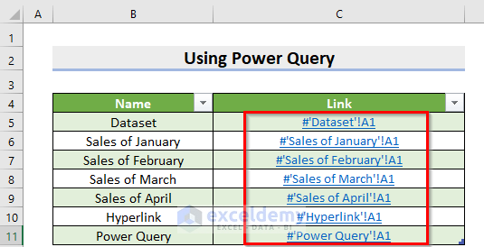
- Create the link for other worksheets.
You will see the following Table of Contents.
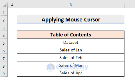
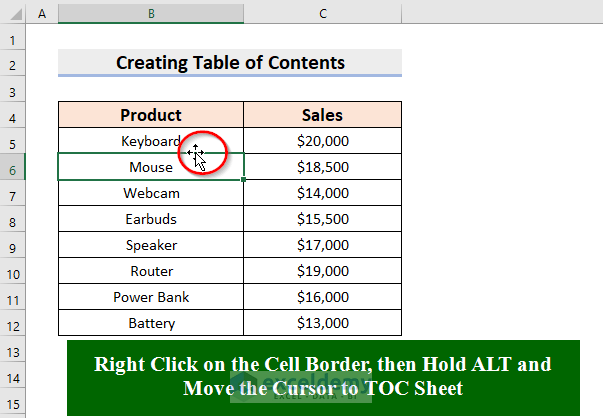
Method 3 – Using the Mouse Cursor to Create a Table of Contents in Excel
Steps:
- Write down the Contents.
- Go to the worksheet named Dataset and right-click on any Cell Border. Don’t release the mouse button.
- Hold the Alt. Don’t release the Alt key.
- Move the Cursor to the worksheet where you keep the Contents.
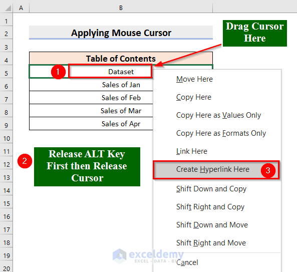
- Bring the Cursor to the corresponding content named Dataset.
- Release the Alt key and then release the Mouse Cursor.
- From the Context Menu Bar, select Create Hyperlink Here
We have attached a GIF.
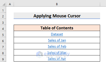
- Create links for other sheets.
Method 4 – Applying Keyboard Shortcuts
Steps:
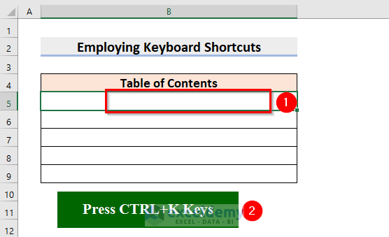
- Select a cell B5 where you want to see the contents.
- Press Ctrl + K.
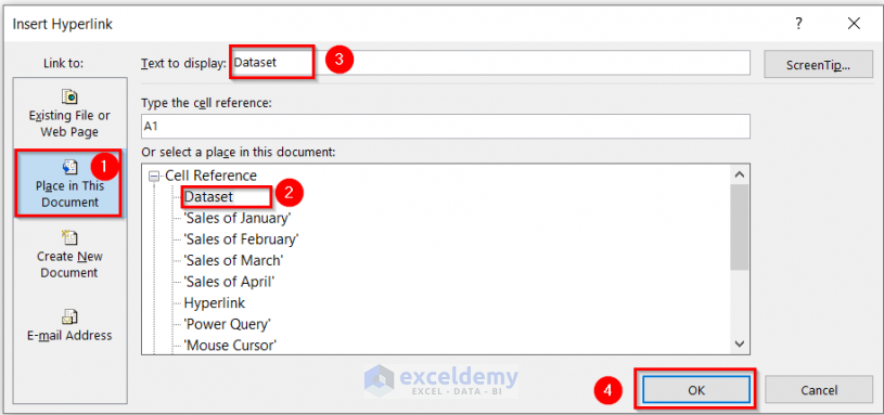
A dialog box named Insert Hyperlink will appear.
- From the Place in This Document command, select Dataset under the Cell Reference.
- Write down what you want to see as content in the Text to display/ We have written “Dataset “.
- Press OK.
You will see the following Content with a link.
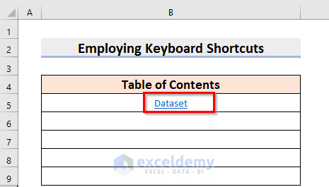
- Similarly, create the link for other worksheets.
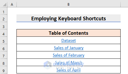
You will see the following Table of Contents.
Read More: How to Create Table of Contents Automatically in Excel
Method 5 – Use the Context Menu Bar to Create the Table of Contents in Excel
Steps:
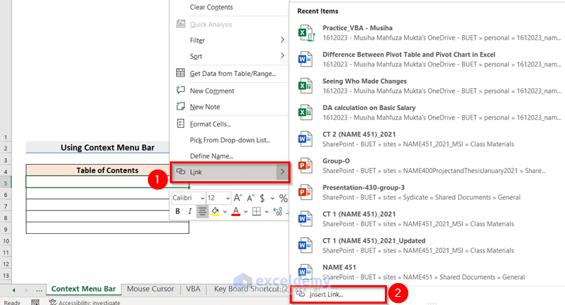
- Select a different cell B5 where you want to see the contents and right-click on it.
- From the Context Menu Bar, choose the Link feature, then select the Insert Link
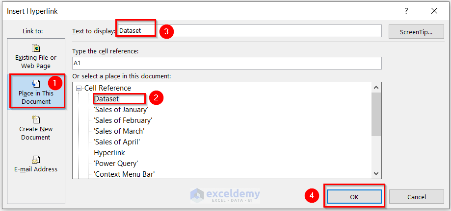
A dialog box named Insert Hyperlink will appear.
- From the Place in This Document tab, select Dataset under the Cell Reference.
- Write down what you want to see as content in the Text to display. We have written “ Dataset “.
- Press OK.
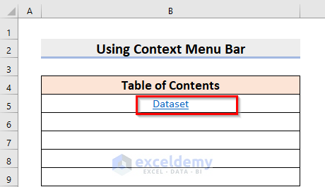
You will see the following Content with a link.
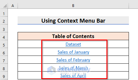
- Create the link for other worksheets.
You will see the following Table of Contents.
Read More: How to Create Table of Contents for Tabs in Excel (6 Methods)
Method 6 – Using VBA Code to Create the Table of Contents
Steps:
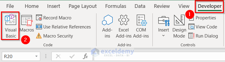
- Choose the Developer tab and select Visual Basic.
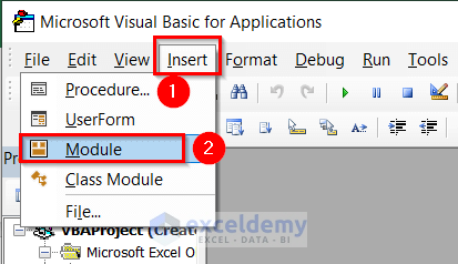
- From the Insert tab, select Module.
- Insert the following Code in the Module.
Sub Table_of_contents()
    Dim Alert_data As Boolean
    Dim numb  As Long
    Dim Sheet_Index As Worksheet
    Dim Sheet As Variant
    Alert_data = Application.DisplayAlerts
    Application.DisplayAlerts = False
    On Error Resume Next
    Sheets("Table of contents").Delete
    On Error GoTo 0
    Set Sheet_Index = Worksheets("VBA")
    numb = 1
    Cells(1, 1).Value = "Table of contents"
    For Each Sheet In ThisWorkbook.Sheets
        If Sheet.Name <> "Table of contents" Then
            numb = numb + 1
            Sheet_Index.Hyperlinks.Add Cells(numb, 1), "", "'" & Sheet.Name & "'!A1", , Sheet.Name
        End If
    Next
    Application.DisplayAlerts = Alert_data
End Sub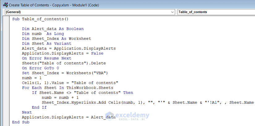
Code Breakdown
- We have created a Sub Procedure named Table_of_Contents.
- We declared some variables Alert_data as Boolean; numb as Long; Sheet_Index as Worksheet; Sheet as Variant.
- If there is any Table of Contents in the active worksheet, the Delete command will delete that.
- We have set the worksheet name as VBA where the Table of Contents will present.
- We used a For Each Loop to include all the worksheets in the Table of Contents.
- Save the code then go back to Excel File.
- Go to the Developer tab and select Macros.
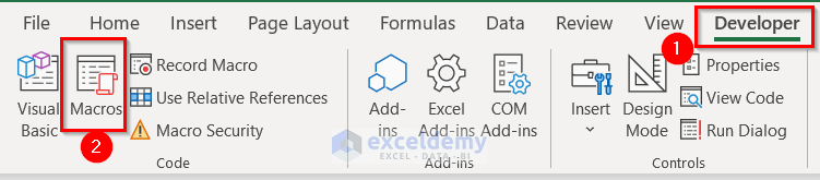
- Select the Macro name (Table_of_Contents) and click on Run.
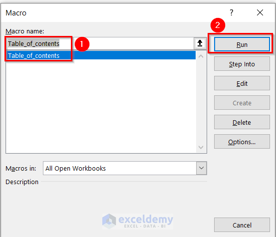
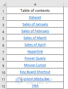
You will see the following Table of Contents which has all the worksheets.
Read More: How to Make Table of Contents Using VBA in Excel (2 Examples)
Download the Practice Workbook

