A dynamic table of contents in Excel allows users to create an interactive and automated index for their workbooks. By linking sheet names and hyperlinks, it enables easy navigation within large Excel files, providing a convenient way to organize and access data, improving efficiency and user experience.
In this article, we will describe how to create a dynamic table of contents in Excel. Here is an overview:
Download Practice Workbook
How to Create Dynamic Table of Contents in Excel: 3 Easy Methods
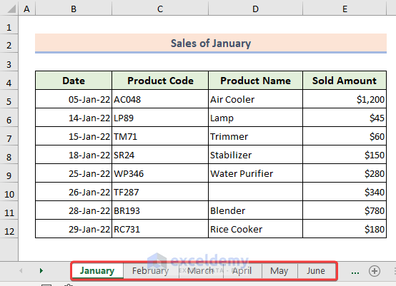
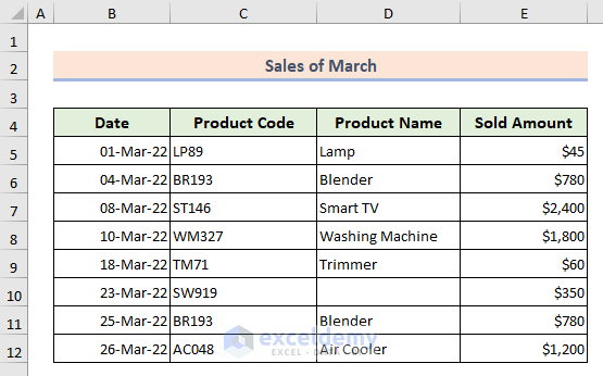
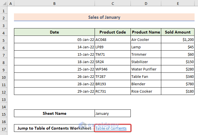
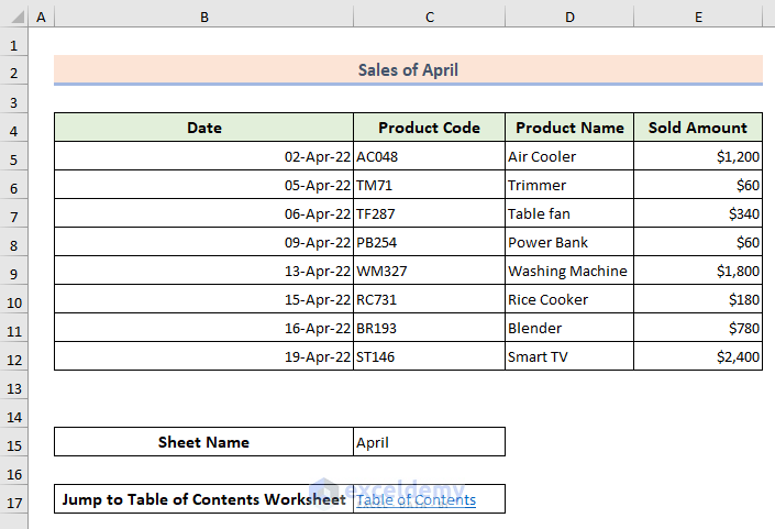
Suppose we have a dataset of a shop’s sales, with each month’s sales in its own worksheet. Let’s create a dynamic table of contents for these multiple worksheets.
Method 1 – Combining the GET.WORKBOOK, HYPERLINK, INDEX, REPLACE, FIND, T, and NOW Functions
The main advantages of this approach are automatic updates and clickable links for easy access.
Steps:
- Create a new worksheet in which to place the table of contents.
We’ll define a name for ease of use within our formulas.
- Click Name Manager from the Formulas tab.
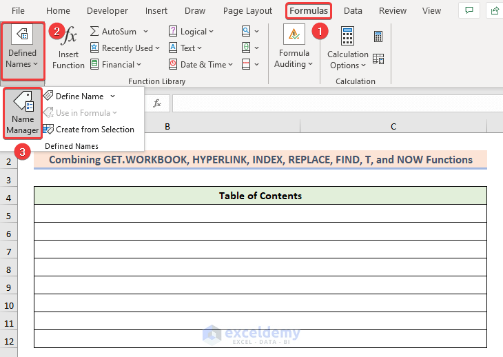
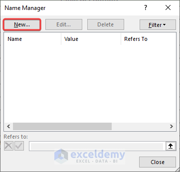
- Select New in the Name Manager window.
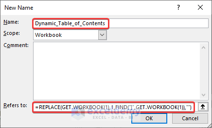
- In the Name section, put your own choice of name.
- In the Refers to section, enter the following formula:
=REPLACE(GET.WORKBOOK(1),1,FIND("]",GET.WORKBOOK(1)),"")
Formula Breakdown:
- GET.WORKBOOK(1)
Retrieves the name of the currently open workbook. Argument 1 specifies the workbook name type.
- FIND(“]”, GET.WORKBOOK(1))
Locates the position of the closing square bracket (“]”) within the workbook name obtained from GET.WORKBOOK(1).
- REPLACE(GET.WORKBOOK(1), 1, FIND(“]”, GET.WORKBOOK(1)), “”)
Replaces the portion of the workbook name string obtained from GET.WORKBOOK(1) starting from the first character and extending to the position of the closing bracket (found using FIND). The replacement is an empty string (“”).
- Close the Name Manager box.
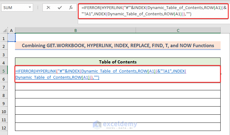
- In cell B5, enter the following formula:
=IFERROR(HYPERLINK("#'"&INDEX(Dynamic_Table_of_Contents,ROW(A1))&"'!A1",INDEX(Dynamic_Table_of_Contents,ROW(A1))),"")
Formula Breakdown:
- ROW(A1):
Returns the row number of Cell A1.
- INDEX(Dynamic_Table_of_Contents,ROW(A1))
Retrieves the value from the Dynamic_Table_of_Contents array based on the row number of cell A1.
- INDEX(Dynamic_Table_of_Contents, ROW(A1))&”‘!A1″ :
Appends the retrieved value from the previous step with the text “‘!A1”. This is used to construct a reference to cell (A1) in a specific sheet.
- “#'”&INDEX(Dynamic_Table_of_Contents,ROW(A1))&”‘!A1” :
Concatenates the “#” symbol, then retrieves the value from the first step (sheet name), and the “‘!A1” reference to form a complete hyperlink destination.
- HYPERLINK(“#'”&INDEX(Dynamic_Table_of_Contents,ROW(A1))&”‘!A1″,INDEX(Dynamic_Table_of_Contents,ROW(A1))),””) :
Creates a clickable hyperlink. The first argument is the constructed hyperlink destination from the previous step, and the second argument is the display text for the hyperlink.
- IFERROR(HYPERLINK(“#'”&INDEX(Dynamic_Table_of_Contents,ROW(A1))&”‘!A1”,INDEX(Dynamic_Table_of_Contents,ROW(A1))), “”) :
Finally, the IFERROR function is used to handle any errors that may occur. It attempts to create a hyperlink using the HYPERLINK function. If an error occurs, such as if the sheet name is not found in the “Dynamic_Table_of_Contents” array, it returns an empty string (“”).
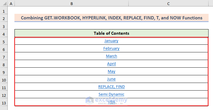
- Press ENTER.
The dynamic table of contents is created.
- To check it works properly, simply click any of the hyperlinks on the sheet.
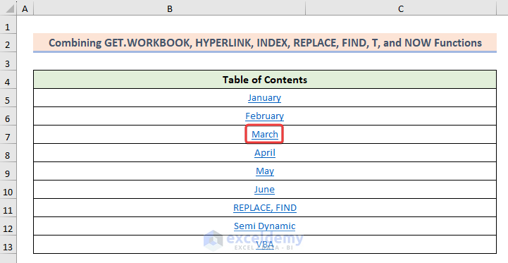
It should take you to the relevant worksheet.
You can also change the worksheet name and it will automatically update in the table of contents wall. For example, here, we changed the worksheet name from “February” to “Feb”.
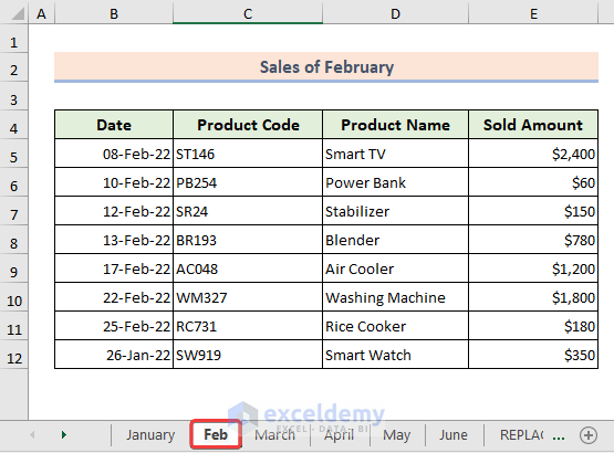
In the table of contents sheet, the worksheet name has changed, confirming the successful creation of a dynamic table of contents.

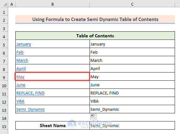
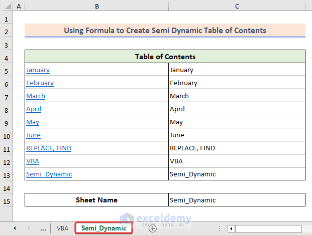
Method 2 – Using a Formula to Create a Semi-Dynamic Table of Contents
We can also create a semi-dynamic table of contents by combining the CELL, TEXTAFTER, VSTACK, and HYPERLINK functions. This approach simplifies maintenance, improves worksheet organization, and automatically updates as sheets are added, deleted, or rearranged.
Steps:
First, we’ll select all the sheets to put the sheet name in a specific location within all the worksheets.
- Holding down the CTRL key, click the left arrow on the left of the Sheet bar.

- Holding down the SHIFT key, click the first worksheet.
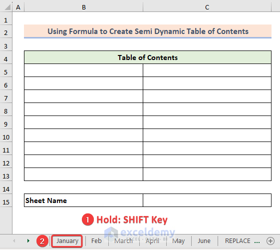
Thus all the sheets will be selected.

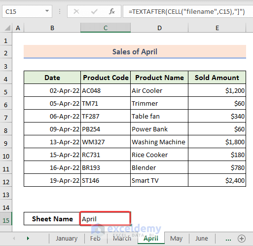
- Select cell C15, enter the following formula, and press Enter:
=TEXTAFTER(CELL("filename",C15),"]")
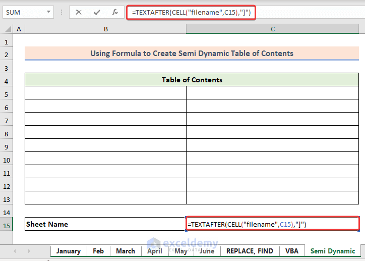
We have the sheet names of all the worksheets in cell C15.
Now we apply the VSTACK function to arrange all the sheet names in one worksheet.
- In cell C5, enter the following formula:
=VSTACK(January:Semi_Dynamic!C15)
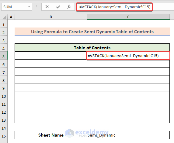
- Pressing ENTER will provide us all the sheet names, like in the image below.

We are ready to link all the sheets with the HYPERLINK function.
- In cell B5, enter the following formula:
=HYPERLINK("#'"&C5&"'!A1",C5)
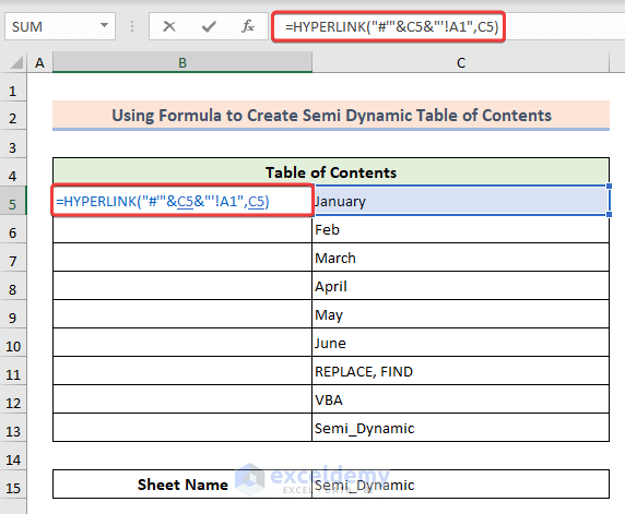
We have successfully created a (semi-)dynamic table of contents in Excel.
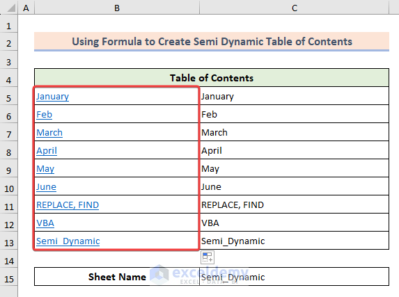
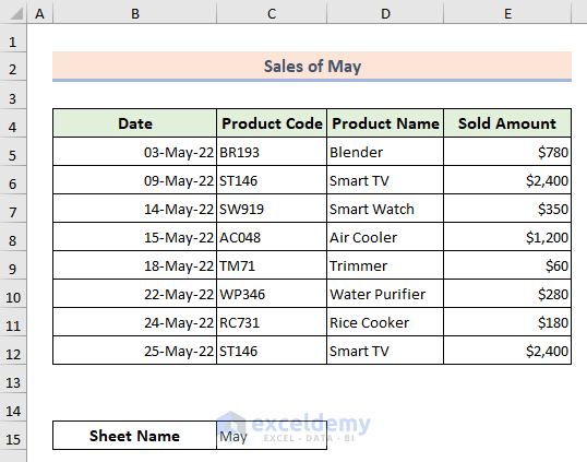
- To check whether it’s working properly, simply click any linked content in the table.
Immediately you will jump to the corresponding worksheet.
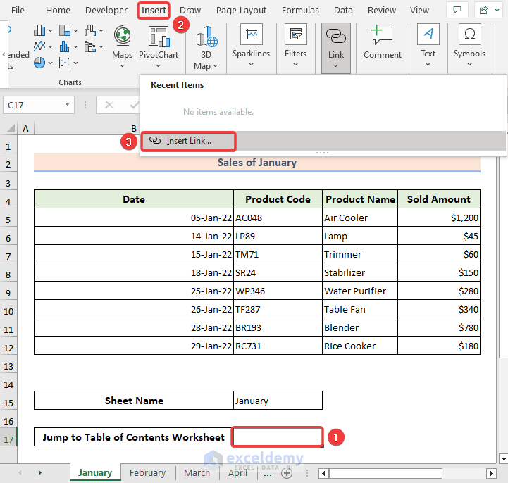
For added convenience, we can add the main table of contents sheet to all the worksheets, so that we can jump back to the main content sheet with a single click from any sheet.
- Select cell C17.
- Click Insert Link from the Insert tab.
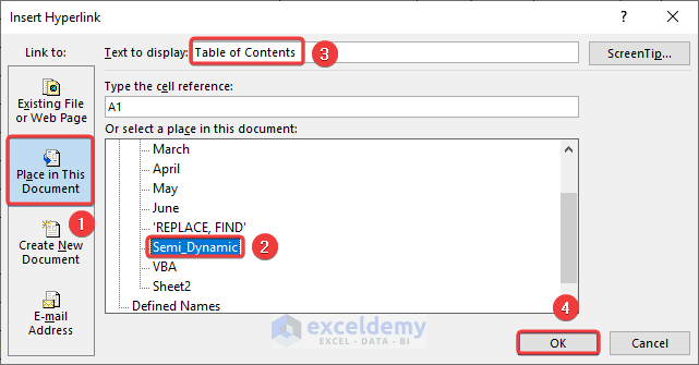
- Choose the table of contents sheet where all the sheet names are located.
- Put your own choice of name in the Text to display section.
- Click OK.
In this whis way, we have added the link to the table of contents sheet.
- Check it by clicking the newly created link.
Within a blink of an eye, we have moved to the table of contents sheet.
- To copy this linked cell to all the worksheets, simply press CTRL+C to copy.
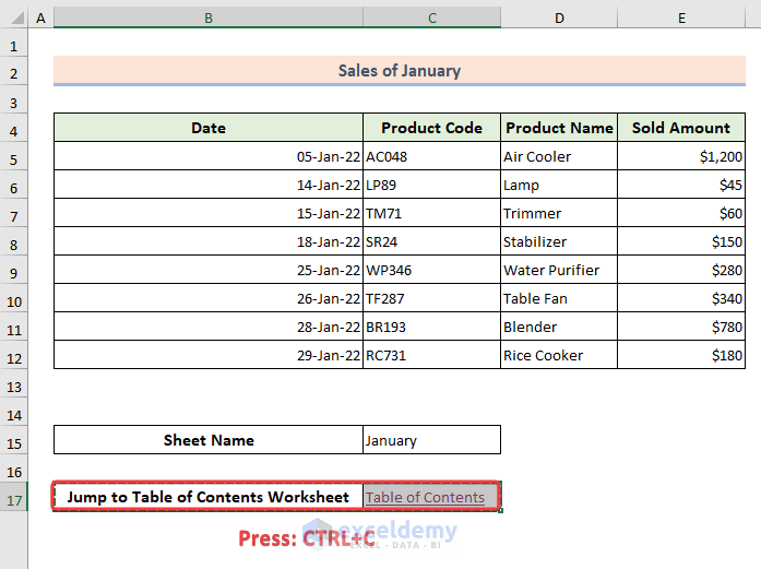
- Just like in the previous steps, select all sheets from the workbook, choose cells B17:C17, and press CTRL+V to paste.
- Make sure the chosen cells are blank for all the sheets, otherwise it won’t work.
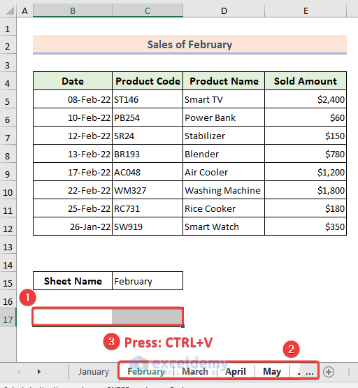
Our linked cells are copied to each worksheet.
Method 3 – Using a VBA Macro to Insert a Dynamic Table of Contents
The main purpose of inserting a dynamic table of contents is to provide a convenient way to navigate through a document’s structure and quickly access specific sections. By applying VBA code, we can automate the table of contents. After applying the code, the table will automatically update whenever changes are made to the workbook.
Steps:
- Follow this link to open the VBA window and insert a module.
- Inside the module, place the below code and click the Save icon:
Sub Dynamic_table_of_contents()
xAlerts = Application.DisplayAlerts
Application.DisplayAlerts = False
On Error Resume Next
Set Sheet_TOC = Sheets("VBA")
On Error GoTo 0
If Sheet_TOC Is Nothing Then
Exit Sub
End If
I = 4
For Each WS In ThisWorkbook.Sheets
If WS.Name <> "VBA" Then
I = I + 1
Sheet_TOC.Hyperlinks.Add Sheet_TOC.Cells(I, 2), "", "'" & WS.Name & "'!A1", , WS.Name
End If
Next
Application.DisplayAlerts = xAlerts
End Sub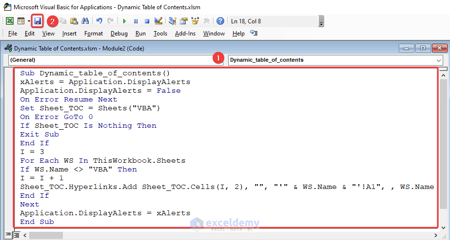
- Insert the following code with a private sub inside the sheet.
- Don’t forget to change to Worksheet and Activate to run your VBA code properly.
Private Sub Worksheet_Activate()
Dynamic_table_of_contents
End Sub
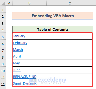
After running the code, our automated table of contents is successfully created
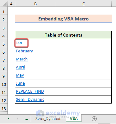
- To check that it’s working properly, change the name of the worksheet from January to Jan.
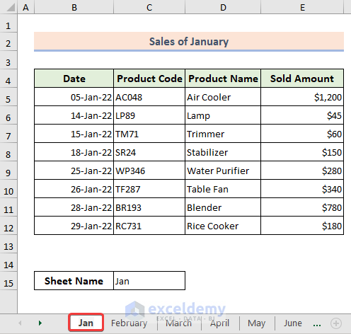
In the main table of contents, the name has changed automatically.
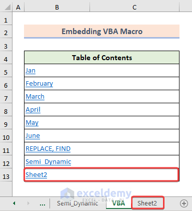
- Add another worksheet by clicking the plus (+) icon on the Sheet bar like in the image below.
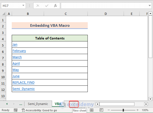
As the new sheet is created, the table of contents updates to include the new sheet in the list automatically.
Things to Remember
- When creating multiple sheets, ensure that the sheet names used in the table of contents match the actual sheet names in your workbook. Any discrepancies can lead to broken links and errors.
- If you plan to dynamically update the table of contents, as you add or remove sheets be mindful of maintaining a consistent sheet order and structure.
Frequently Asked Questions
Can I automatically update the Table of Contents when I add or remove sheets in my workbook?
Yes, you can set up the table of contents to automatically update by using dynamic formulas, such as INDEX and INDIRECT.
Is it possible to customize the appearance and formatting of the table of contents?
Yes, by applying formatting styles, changing font sizes, adding colors, and modifying cell borders.
Can I create a hierarchical or nested table of contents with multiple levels?
Yes, by using indentation or multiple columns.
Get FREE Advanced Excel Exercises with Solutions!


I tried method One, and it is not dynamic. Even when I close excel and restart, or refresh the workbook…..any updates I did to worksheet names are not updated. Any ideas why it is not working?
Hello Anne,
You’re right, Method 1 is not truly dynamic in real-time because it uses a named range based on the old GET.WORKBOOK function, which only updates when you force a full recalculation of the workbook. Simply refreshing or closing and reopening Excel usually isn’t enough.
Try pressing Ctrl + Alt + F9 to force a complete recalculation.
Alternatively, you can manually edit any cell (even just type and delete) to trigger an update.
For a fully automatic update without manual recalculation, you might prefer Method 3 (VBA Macro), as it dynamically rebuilds the Table of Contents whenever a change happens.
Regards
ExcelDemy