Looking for ways to know how Excel hides columns based on cell value without a macro? Sometimes, we want to hide columns based on cell value. We can do it by both using macro and without using macro. Here, you will find step-by-step explained ways to Excel hide columns based on cell value without a macro.
Excel Hide Columns Based on Cell Value without Macro: 2 Steps
Here, we will show you how Excel hides columns based on cell value without a macro by going through 2 steps: Making a Dataset and using the Conditional Formatting feature. Follow the steps given below to do it on your own.
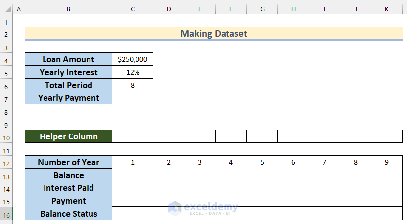
Step-01: Making Dataset to Hide Columns Based on Cell Value
Firstly, we will make a dataset to hide columns based on cell value. Go through the steps to do it yourself.
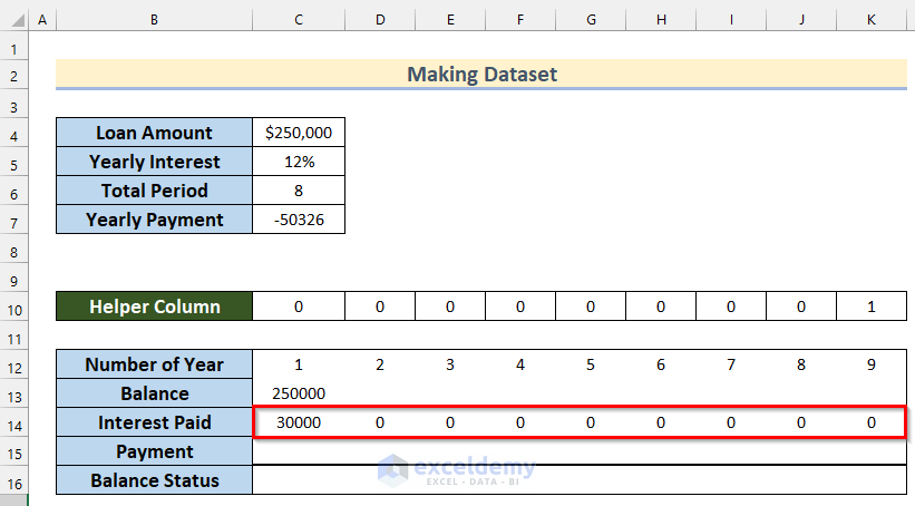
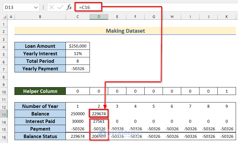
- In the beginning, insert data according to your preference for Loan Amount, Yearly Interest, and Total Period. Here, we will insert $250,000 as the Loan Amount, 12% as Yearly Interest, and 8 as the Total Period.
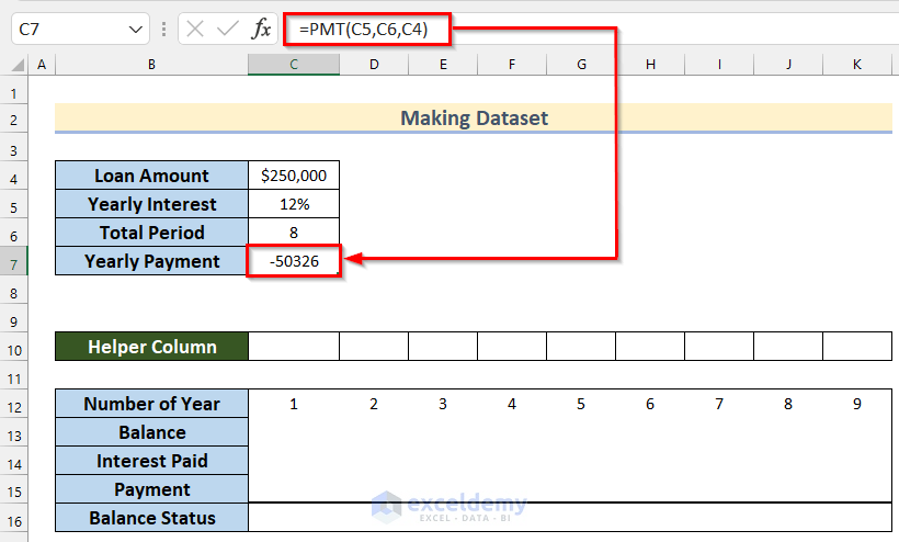
- Then, select Cell C7.
- Next, insert the following formula.
=PMT(C5,C6,C4)
Here, we used the PMT function to calculate the value of the Yearly Payment. Now, in the PMT function, we selected Cell C5 as rate, Cell C6 as nper, and Cell C4 as pv.
- Now, press ENTER.
- After that, select Cell C10.
- Then, insert the following formula.
=IF(C$12<=$C$6,0,1)
Here, we used the IF function to check if the value of the Number of Year is less than or equal to the Total period. Then, If it is TRUE then the function will return 0, or else it will return 1.
- Next, press ENTER.
- Afterward, drag right the Fill Handle tool to AutoFill the formula for the rest of the cells.

- Now, you will get all the values of the Helper Column using the IF function.

- Then, select Cell C13.
- After that, insert the following formula.
=C4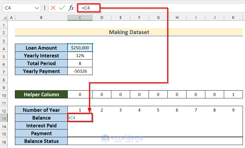
Here, we select the starting Balance as the value of the Loan Amount.
- Next, press ENTER.

- Now, select Cell C14.
- After that, insert the following formula.
=C13*$C$5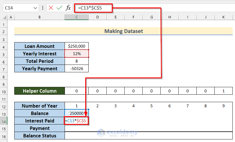
Here, we multiplied the value of the Balance with Yearly Interest to get the value of Interest Paid.
- Next, press ENTER.
- Then, drag right the Fill Handle tool to AutoFill the formula for the rest of the cells.

- Now, all the cells representing the value of Interest Paid will have a suitable equation to calculate their values. The values will change according to the values of the Balance amount.
- Then, select Cell C15.
- After that, insert the following formula.
=$C$7
In this formula, we select the Payment as the value of the Yearly Payment.
- Next, press ENTER.
- Now, drag right the Fill Handle tool to AutoFill the absolute value for the rest of the cells.
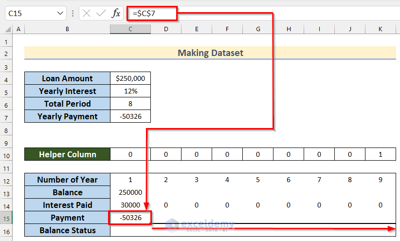
- After that, you will get all the values of the Payment.

- Then, select Cell C16.
- Afterward, insert the following formula.
=SUM(C13:C15)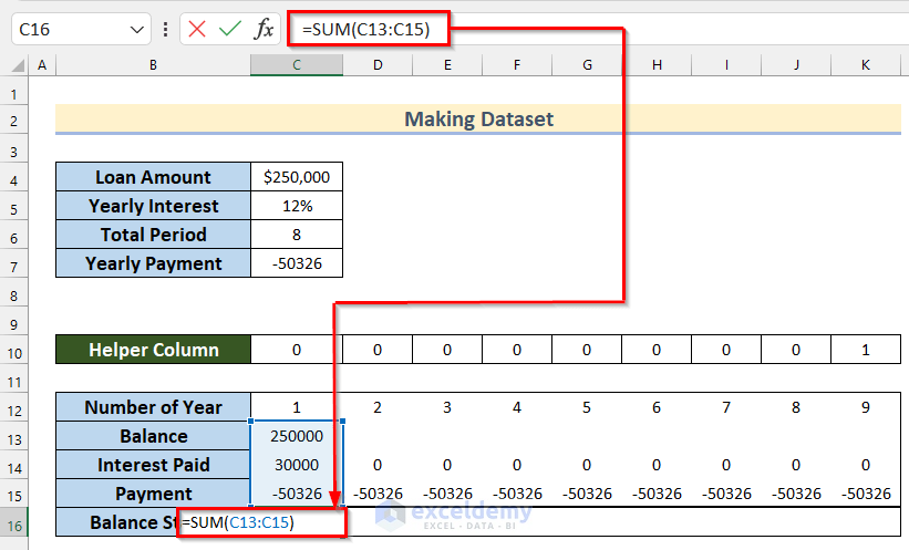
Here, we used the SUM function to add the values of Balance, Interest Paid, and Payment to get the value of Balance Status.
- Next, press ENTER.
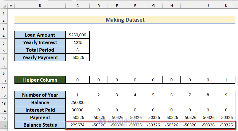
- Now, drag right the Fill Handle tool to AutoFill the formula for the rest of the cells.

- Now, you will get all the values of the Balance Status.
- After that, select Cell D13.
- Then, insert the following formula.
=C16
Here, we select the Balance Status of the 1st year as the value of the Balance of the 2nd year.
- Next, press ENTER.
- Now, you will get the value of the Balance for the 2nd year.
- Additionally, you can see that the values of Interest Paid and Balance Status have also changed according to their corresponding equations.
- After that, insert equations in Cell range E13:J13 so that it returns the values of the Balance Status of their corresponding previous year by going through the steps explained above.
- Finally, you will get all the values of the Balance.
- Additionally, you will see that the values of Interest Paid and Balance Status have also changed according to their corresponding equations.

Read More: How to Hide Columns in Excel with Password
Step-02: Using Conditional Formatting Feature to Hide Columns Based on Cell Value
Now, we will show you how to use the Conditional Formatting Feature to hide columns based on cell values in Excel. Follow the steps given below to do it on your own.
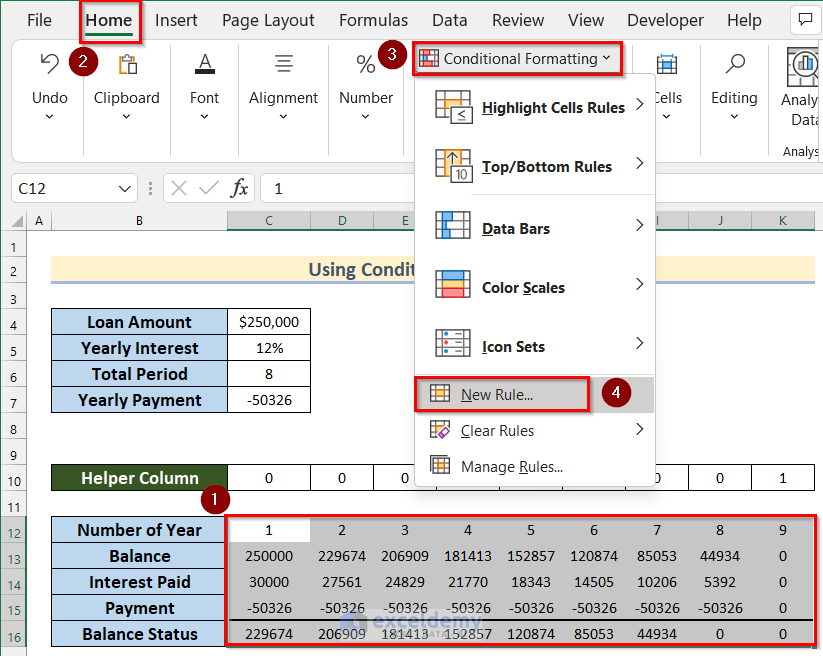
- Firstly, select Cell range C12:K16.
- Then, go to the Home tab >> click on Conditional Formatting >> select New Rule.
- Now, the New Formatting Rule box will appear.
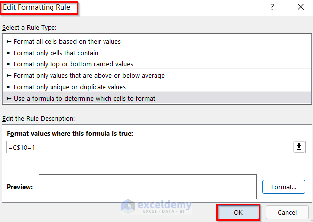
- Next, select Use a formula to determine which cell to format as Rule Type.
- Then, type =C$10=1 in the Format values where this formula is true box. Here, we fixed Row 10 by using $ sign so that the formula can be used for the Cell range C10:K10. Now, If the Cell value is equal to 1, then the provided format will work on the cell.
- After that, click on Format.

- Now, the Format Cells box will open.
- Next, go to the Font option >> click on Color box >> select White, Background1.
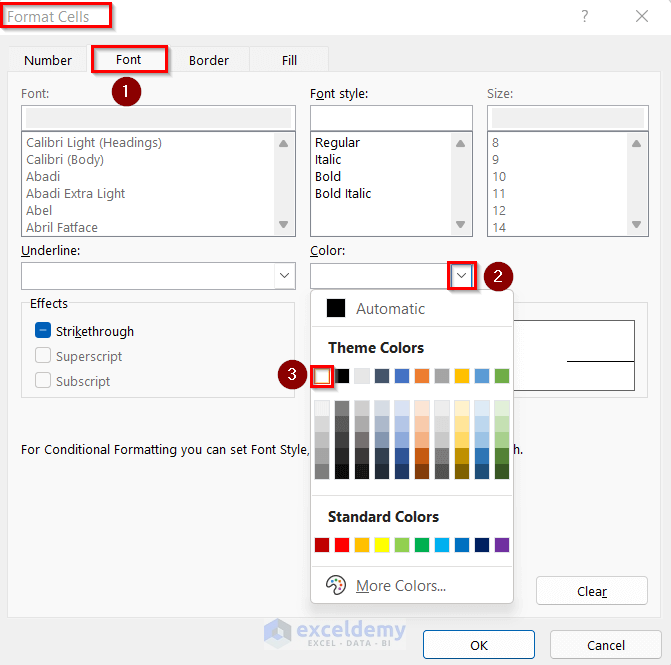
- Then, go to the Border option >> select None.
- After that, press OK.

- Now, the Edit Formatting Rule box will appear.
- Next, press OK.
- After that, you will see that the values of Cell range K12:K16 have been hidden.

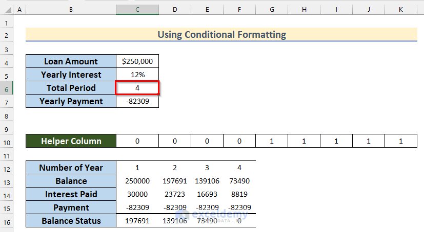
- Then, to check the formatting properly change the value of Cell C4 as 4.
- Finally, you will see that several columns have been hidden based on the cell value of the Total Period.
Read More: How to Hide Columns in Excel with Minus or Plus Sign
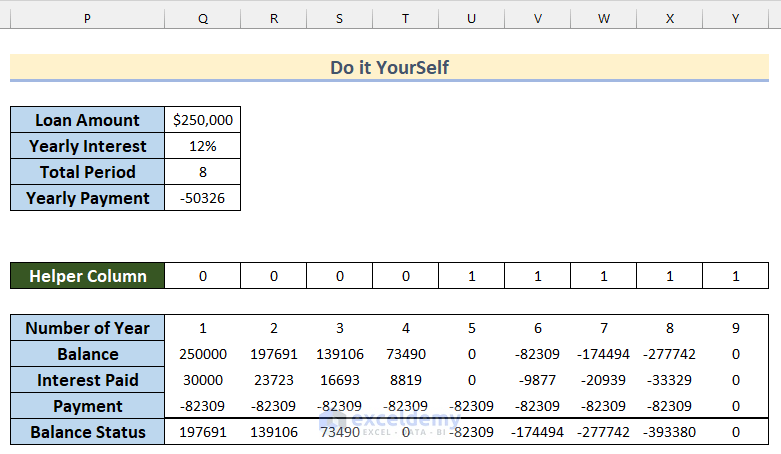
Practice Section
In this section, we are giving you the dataset to practice on your own and learn to use these methods.
Download Practice Workbook
Conclusion
So, in this article, you will find a step-by-step way Excel hides columns based on cell value without a macro. Use any of these ways to accomplish the result in this regard. Hope you find this article helpful and informative. Feel free to comment if something seems difficult to understand.
Related Articles
- How to Hide Selected Columns in Excel
- How to Group and Hide Columns in Excel
- How to Collapse Columns in Excel
<< Go Back to Hide Columns | Columns in Excel | Learn Excel
Get FREE Advanced Excel Exercises with Solutions!
