How to Hide Columns in Excel with Minus or Plus Sign: 2 Methods

Method 1 – Hide Columns with Plus Sign Using the Group Feature

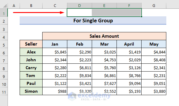
1.1 For Single Group of Columns

STEPS:

• Select the first cells of the columns you want to hide with the help of the mouse. Do not use the Ctrl key to select columns. We selected Cells D1, E1 & F1 to hide Columns D, E & F.

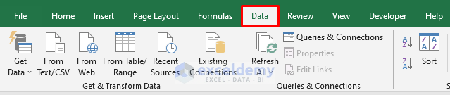
• Go to the Data tab.

• Select Group from the Data A drop-down menu will occur.

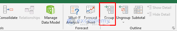
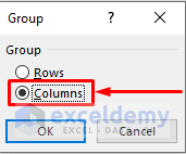
• Select Group from the drop-down menu. The Group window will appear.

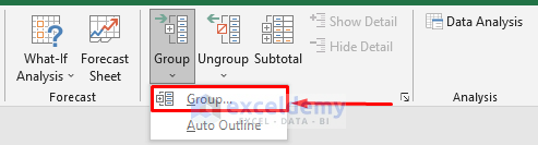
• Choose ‘Columns’ in the Group window.

• A minus sign will appear at the top of the columns we selected to hide, just like below.

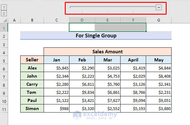
Use the keyboard shortcut to group and ungroup columns. To add grouping, select the range of columns and press Shift + Alt + Right Arrow. To remove grouping, press Shift + Alt + Left Arrow.

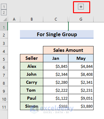
• Click the minus sign to hide the columns like below. If you select the plus sign, then hidden rows will be visible again.

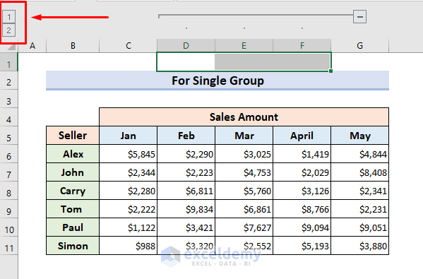
• Clicking 1 will hide the columns, and clicking 2 will unhide the columns.

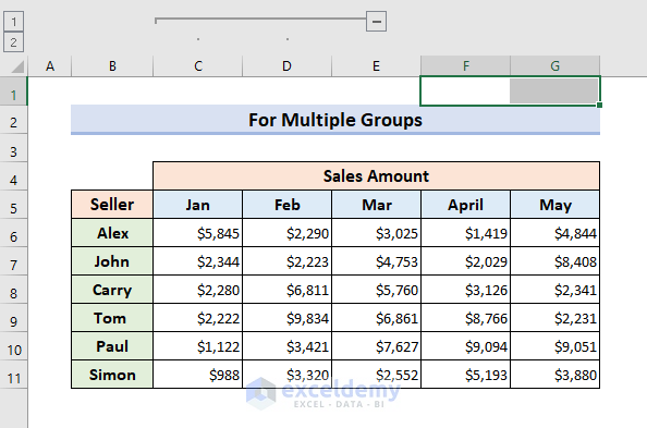
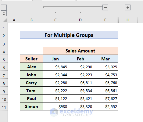
1.2 For Multiple Groups of Columns

STEPS:

• Select the columns you want to group. We selected Columns F & Column G.

• Go to the Data tab and select Group.

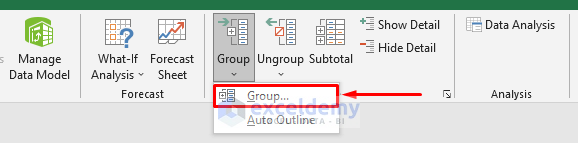
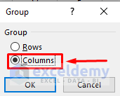
• Select ‘Columns’ from the ‘Groups’ Click OK to proceed.

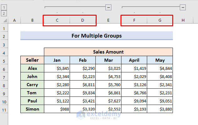
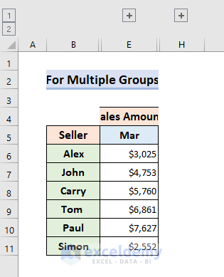
• You will see two groups of columns like below.

• If you click on the minus sign the columns will be hidden and if you click on the plus sign the columns will be visible.

• You can hide both groups of columns like below.

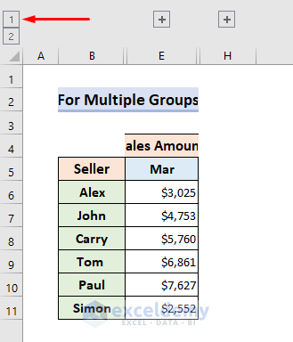
• If you click 1, both columns will be hidden together.

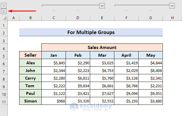
• To unhide them, click 2.

Method 2 – Use of Auto Outline to Hide Columns with Plus Sign

STEPS:

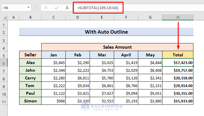
• Select Cell H6 and type the formula:

• Hit Enter and use the Fill Handle to see results in all cells.

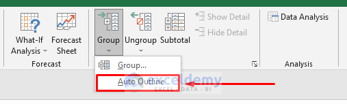
• Go to the Data tab and select ‘Auto Outline’ from the drop-down menu.

• You will see the minus sign above the columns used in the SUBTOTAL Function.

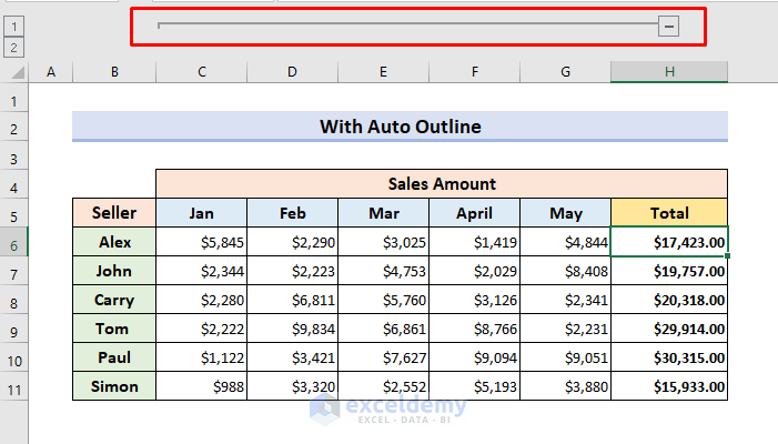
• Click the minus sign to hide it and the plus sign to unhide the columns.

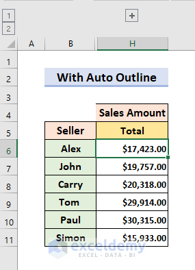
You can also click the 1 & 2 buttons to hide & unhide.

How to Manually Hide Columns in Excel?

STEPS:

• Select the columns you want to hide. You can use the Ctrl key to select multiple columns.

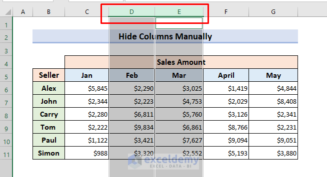
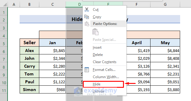
• Place your cursor on the top of Column D and right-click the mouse.
• Hide from the drop-down menu.

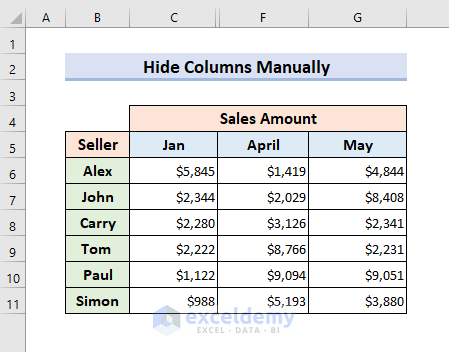
• The columns will be hidden.

Excel Hide Columns Using Keyboard Shortcut

Excel has some keyboard shortcuts to hide/unhide columns that make our job very easy.

• To hide a single column: Select any cell in the column, and then press Ctrl + 0.
• To hide multiple columns: Press Ctrl and select the columns you want to hide. Then, press Ctrl + 0 to hide them.

Download Practice Book

Download the practice book.

Related Articles

• How to Group and Hide Columns in Excel
• How to Collapse Columns in Excel
• Excel Hide Columns Based on Cell Value without Macro

<< Go Back to Hide Columns | Learn Excel