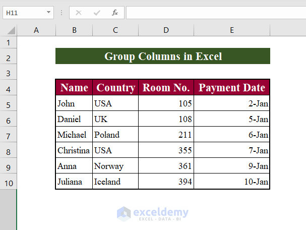
Consider you have data in existing cells that contain names from different countries. They have different room numbers to be allocated according to their payment history. You have to group them into columns to organize a comparable layout.
Steps
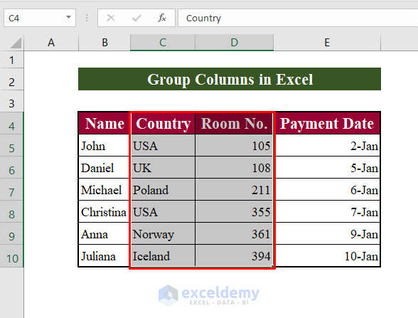
- Select the columns you want to group. In this example, we will select columns C and D.
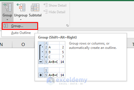
- Select the Data tab from the Ribbon.

- Click on Group.
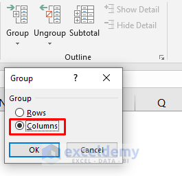
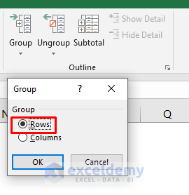
- Select the Columns option and press Enter.
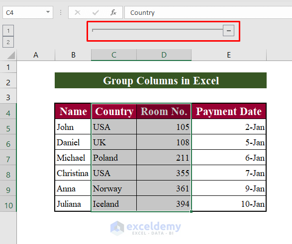
- The selected columns will be grouped. Here, columns C and D are grouped together. You can see the horizontal line marked with a red box.
Read More: How to Group Duplicates in Excel
Read More: How to Group Cells with Same Value in Excel
How to Ungroup Columns
Steps:
- Select the grouped columns.
- Click Ungroup.

How to Hide and Show Grouped Columns in Excel
Steps:
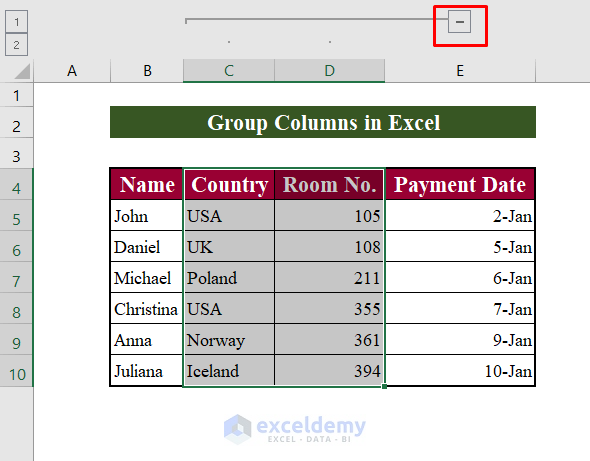
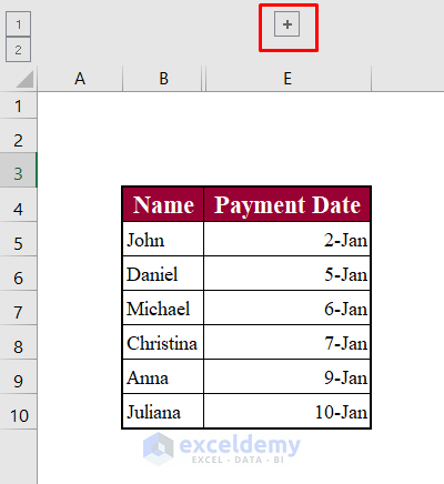
- Click the Hide Detail icon.
- Click the Show Detail button to show the group.
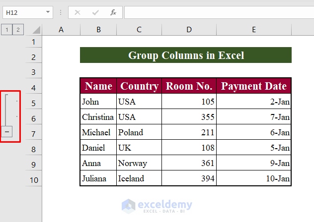
How to Group Rows in Excel
Steps:
- Select the rows you want to group.
- Select Rows from the Group command on the Data tab.
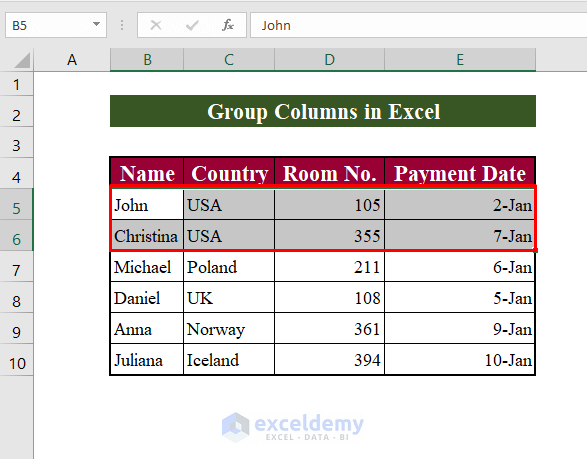
- You will see the grouped rows indicating a vertical line on the left.
Things to Remember
- In your Excel worksheet, you won’t be able to add Calculated Items to grouped Fields.
- It’s impractical to select a few columns that aren’t nearby.
Download the Practice Workbook
Related Articles
- How to Use Grouping and Consolidation Tools in Excel
- How to Create Multiple Groups in Excel
- How to Group Similar Items in Excel
- How to Group Time Intervals in Excel
- How to Remove Grouping in Excel
<< Go Back to Group Cells in Excel | Outline in Excel | Learn Excel
Get FREE Advanced Excel Exercises with Solutions!
