How to Group Cells with Same Value in Excel (3 Methods)

Let’s assume a scenario where we have an Excel file that contains information about the products that a country exports to different countries in Europe. We have the Product name, exported Amount, and the Country to which the product is exported. We will use this worksheet to show you how to group cells with the same value in Excel.

Method 1 – Group Cells with the Same Value in Excel Using the Subtotal Feature

We will group all the cells with same value in the Country column.

Steps:

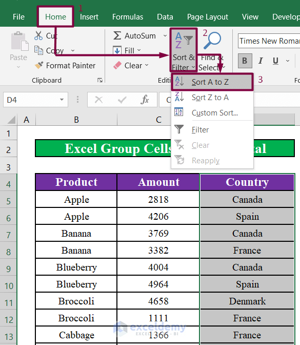
Select all the cells in the Country column.
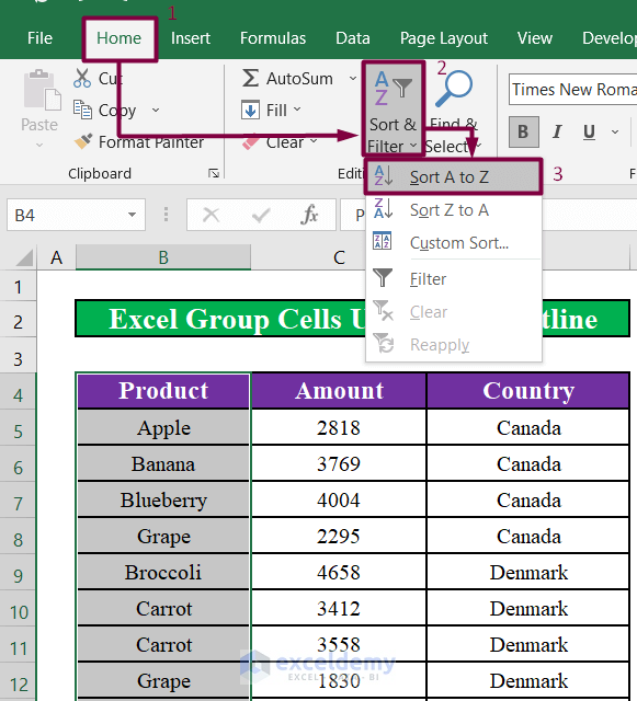
Click on the Sort and Filter drop-down menu from the Editing section under the Home tab.
Select Sort A to Z from the Sort and Filter drop-down.

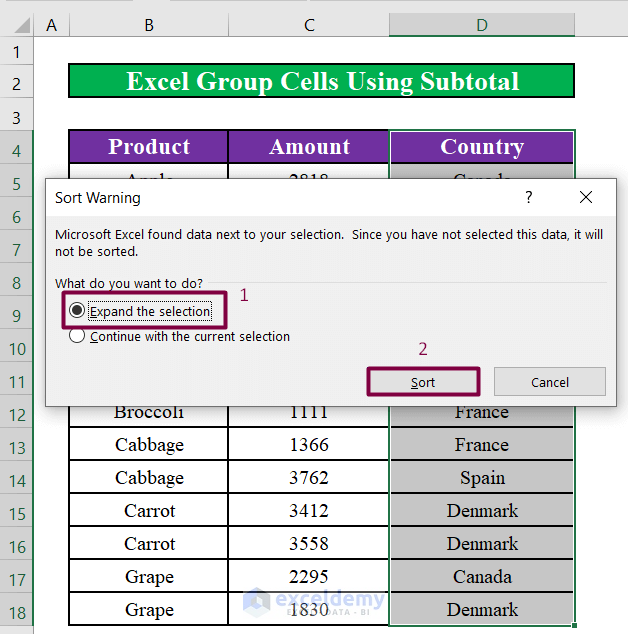
A window named Sort Warning will appear to ask if you want to select the next to our selection. Select Expand the selection.
Click on Sort.

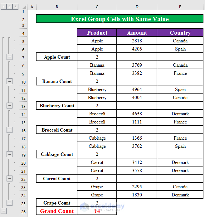
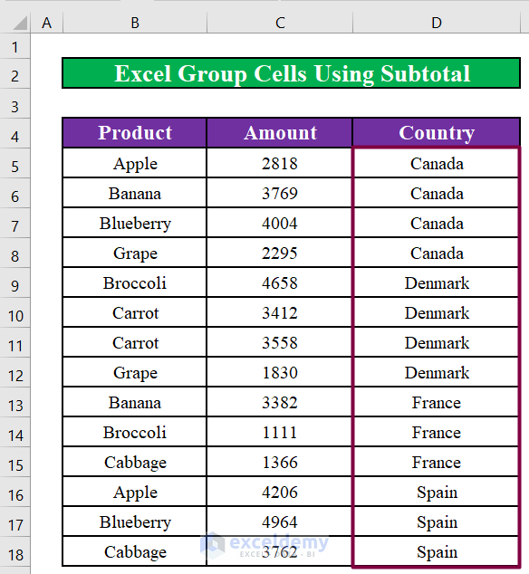
All the cell values in the Country column have been sorted.

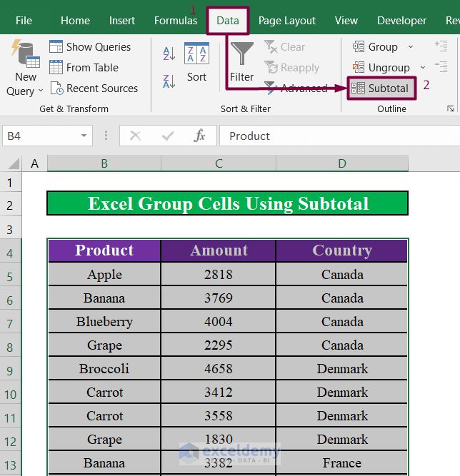
Click on Subtotal from the Outline section under the Data.

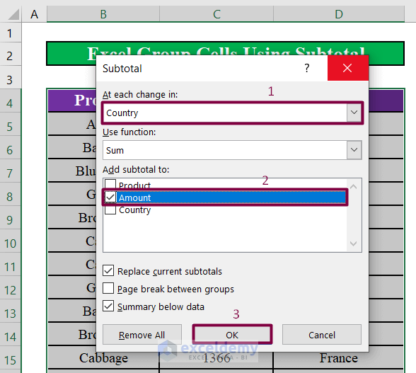
A new window titled Subtotal will appear. Choose Country from the At each change in drop-down.
Only select Amount from Add Subtotal to.
Click on OK.

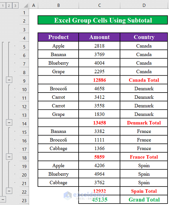
All the rows of the worksheet have been grouped based on the cells with same value in the Country.

Method 2 – Apply the Auto Outline Option to Group Cells with the Same Value in Excel

Steps:

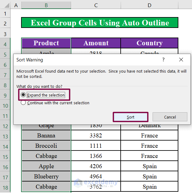
Select all the cells in the Country column.
Click on the Sort and Filter drop-down menu from the Editing section under the Home tab.
Select Sort A to Z from the Sort and Filter drop-down.

A window named Sort Warning will appear to ask if you want to select the next to our selection. Select Expand the selection.
Click on Sort.

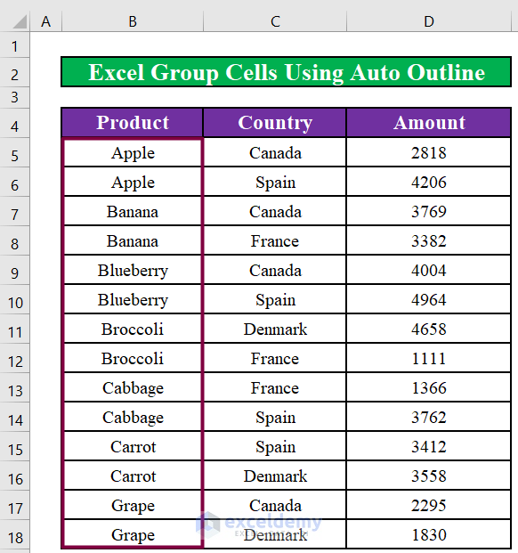
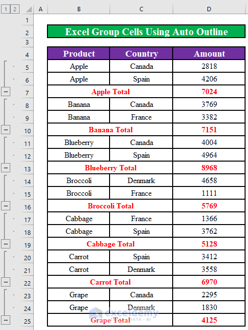
All the cell values in the Product column have been sorted.

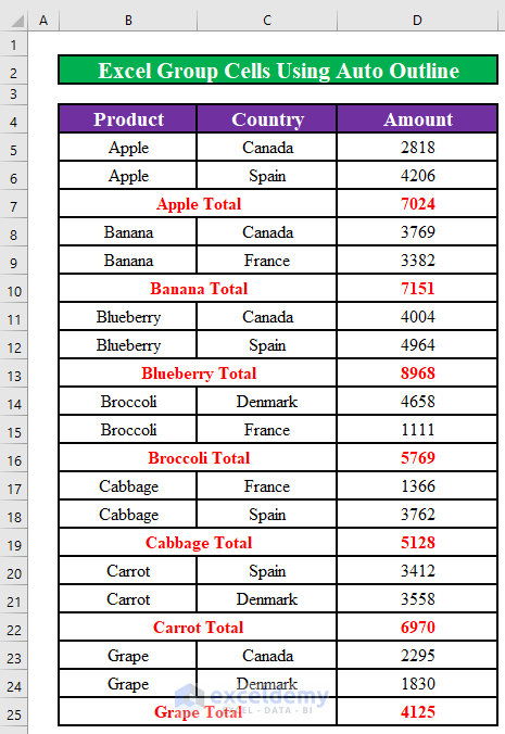
We have also added a new row under each type of product that indicates the total amount of product sold.

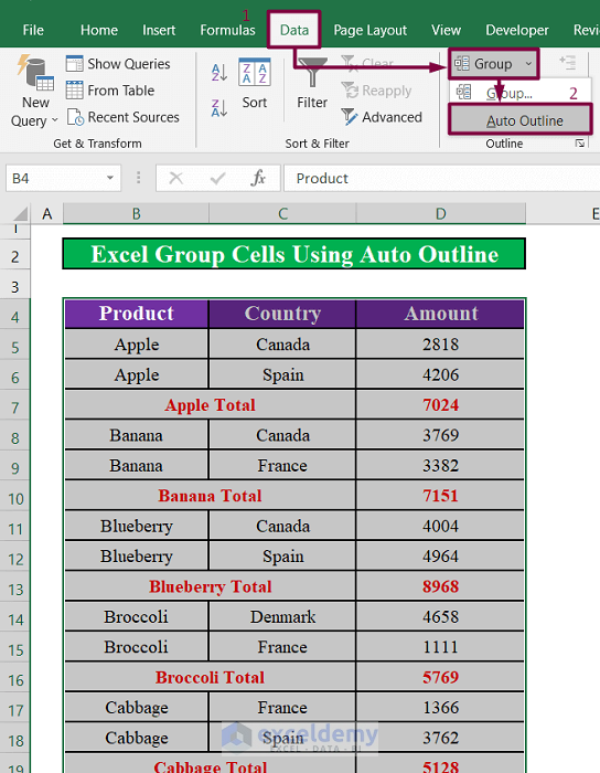
Click on the Group drop-down under Data.
Select Auto Outline from the drop-down menu.

All the rows of the worksheet have been grouped based on the cells with same value in the Product.

Method 3 – Use a Pivot Table to Group Cells with the Same Value in Excel

Steps:

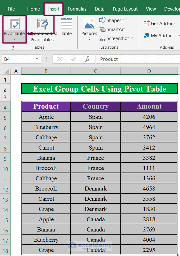
Select all the cells with the data including the column header.
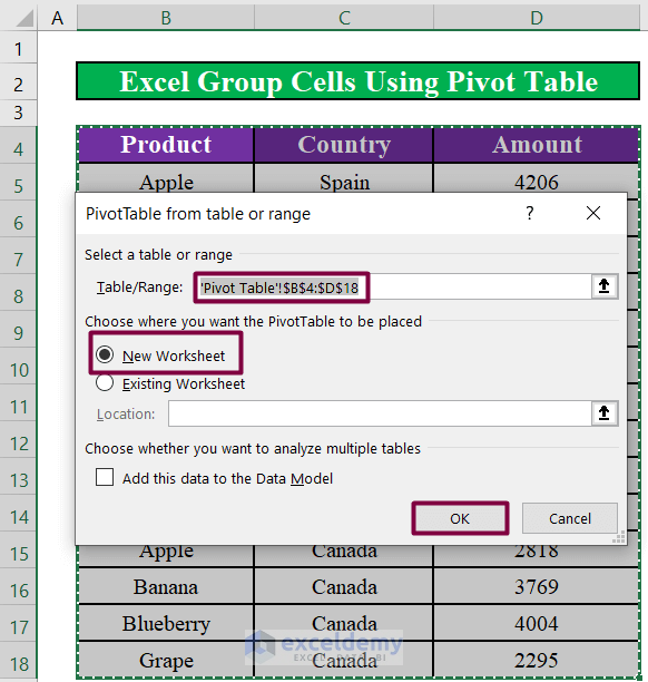
Go to the Insert ribbon and click on PivotTable.

A dialog box will appear. Excel will automatically select the dataset for you. For the new pivot table, the default location will be a New Worksheet.
Click OK.

A new sheet will appear. It will have a box on the right side of the sheet titled PivotTable Fields. You will find it on the left side of the sheet if you are working with Excel 2007/2010.

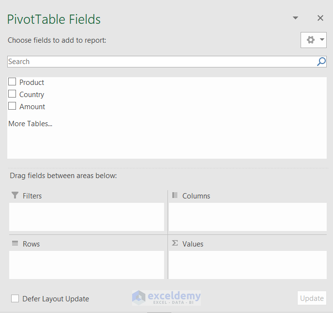
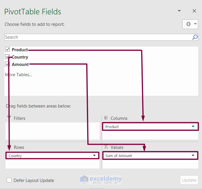
Drag and drop fields from your data like the image below.
- Product fields to the Columns.
- Country fields to the Rows.
- Amount field to the Values.

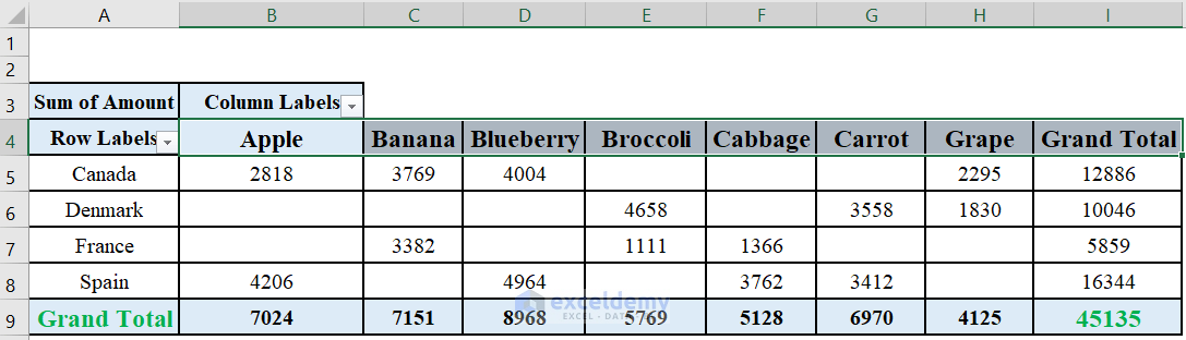
Excel has created a pivot table that groups all the cells with the same value.

Quick Notes

You have to sort the cells in your Excel worksheet before you can use the Subtotal or Auto Outline feature in Excel.
The pivot table will always sort the information in an alphabetically ascending order by default. You have to use the sort option to reorder the information.
Select New Worksheet when you are creating a pivot table. If you select Existing Worksheet, a pivot table will be created in your existing sheet that contains the data. You can distort your dataset if you create the pivot table in an existing worksheet.

Download the Practice Workbook

Group Cells.xlsx