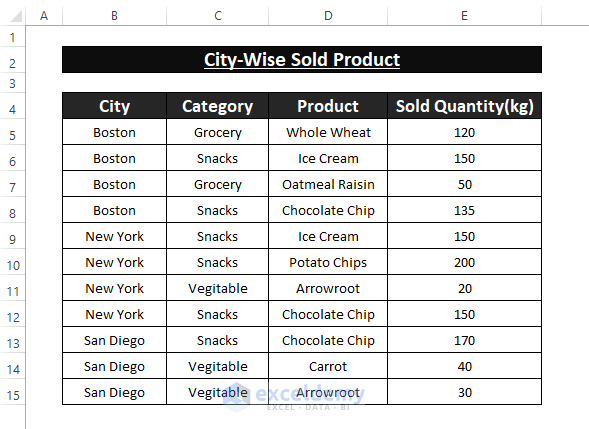
In this article, we demonstrate multiple ways to group rows with same value using Excel features and formulas. Suppose we have an organized dataset containing City wise Product sales. We want to group the rows depending on their row values.
To simplify the process of grouping rows by value, the data should be organized by sorting it first, as it much easier to group organized sorted data. In case of unorganized data, execute a Custom Sort by going to Home > Sort & Filter > Custom Sort.
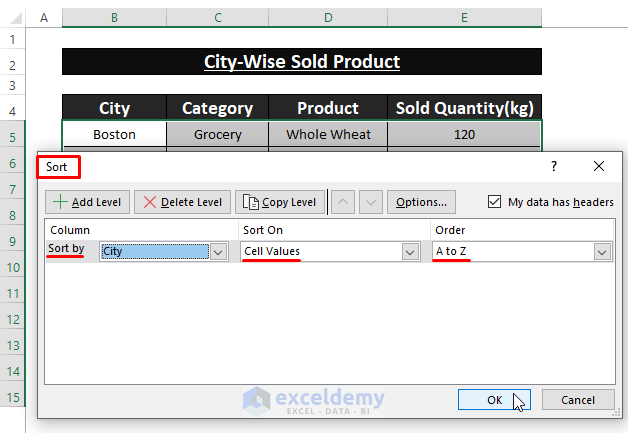
From the Sort window, choose any Column Heading (e.g. City) as the Sort by option.
Method 1 – Using Subtotal Feature to Group Rows with Same Value
The Subtotal feature groups entries, and offers several functions to execute within the groups.
Steps:
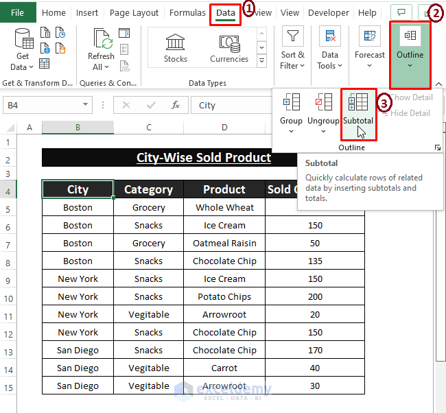
- Place the cursor in any cell within the dataset.
- Go to the Data tab.
- Click on Subtotal (from the Outline section).
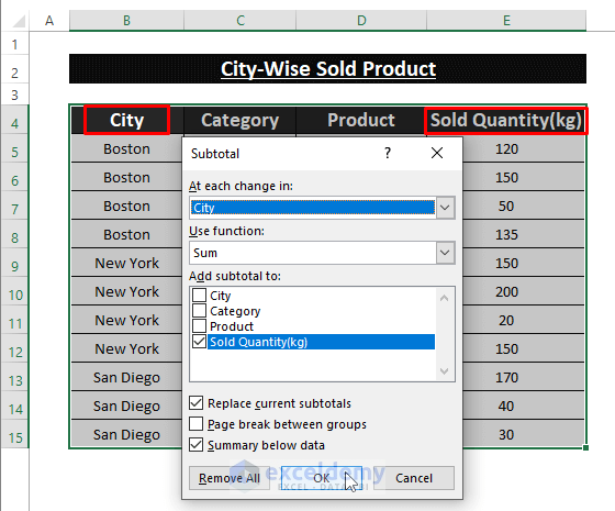
The Subtotal window appears.
- Choose City as At each change in.
- Select any function offered in Use Function drop-down box.
- Tick the column in which to Add Subtotal To.
- Enable other options as desired.
- Click on OK.
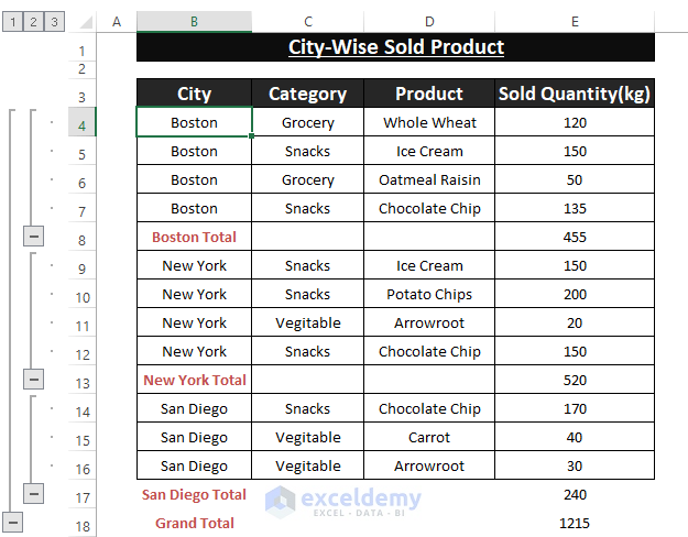
Excel groups our rows depending on their values with a Subtotal for each group, as in the below picture.
Hide any groups by clicking the Minus (–) icon on the left side of the dataset. There are 3 separate groups of rows showing 3 different prioritized items. Above the dataset, there are also 3 different prioritized display options that showcase the different levels of grouping (i.e., 1,2,3).
Read More: How to Group Rows by Cell Value in Excel
Method 2 – Auto Outline Data to Group Rows with Same Value
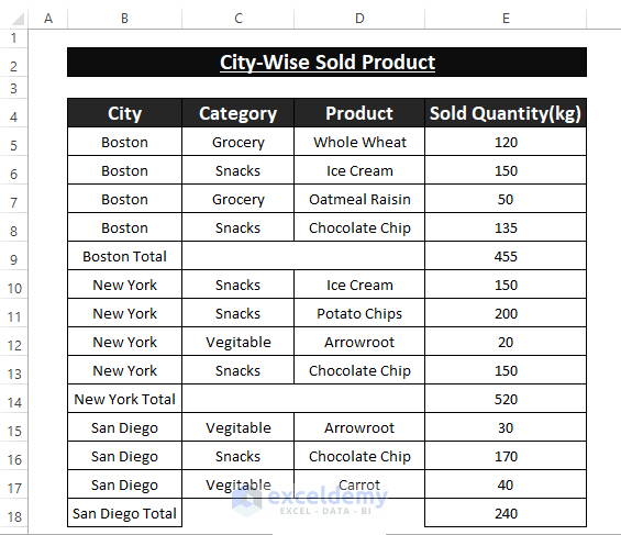
Suppose, as in the following screenshot, that our data is already categorized with Subtotals, and we now want to differentiate between our groups.
Steps:
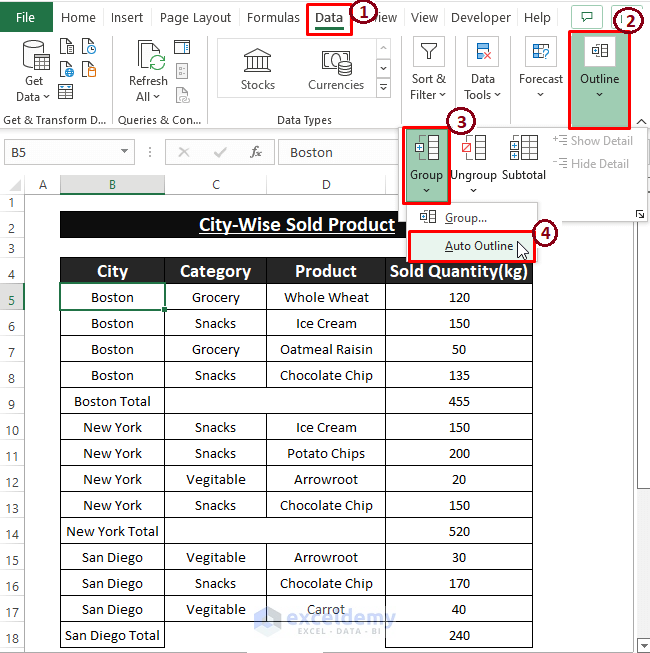
- Go to the Data tab.
- Click on Group (from the Outline section).
- Click on Auto Outline.
Without organized data Auto Outline will not work. The data must be in sections with similar data types but different entries.
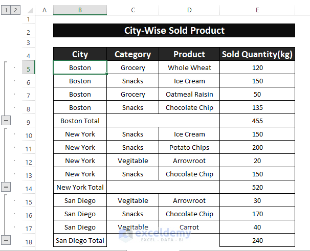
Excel forms 3 groups, since we have 3 different categories.
Read More: How to Group and Ungroup Columns or Rows in Excel
Method 3 – Using Group Feature to Manually Group Rows
Grouping entries in the dataset can be intense when we categorize many entries. To group rows by more than 1 criterion, we need to execute nested grouping, which can only be done manually.
Single Grouping:
Before being able to create a nested grouping, we need to Group Rows for an outer sphere.
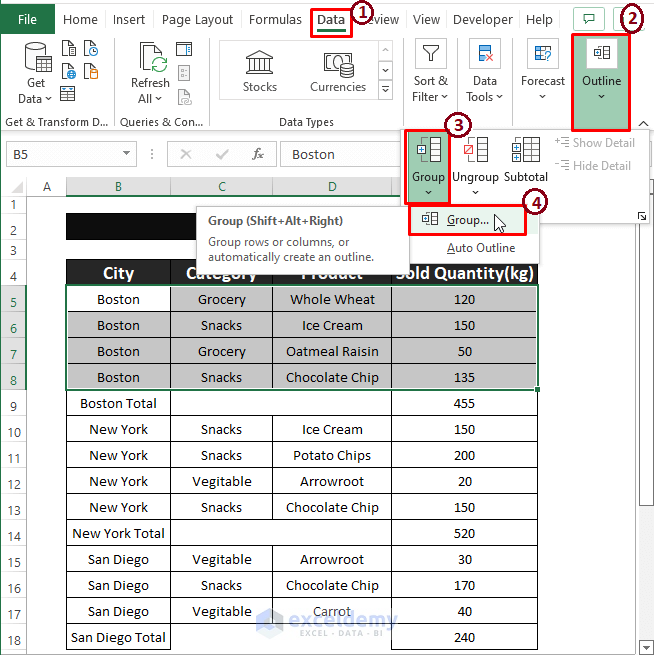
Steps:
- Select the outer group rows.
- Go to the Data tab.
- Click on Group (from the Outline section).
- Click Group.
The Group dialog box appears.
- Choose Rows.
- Click on OK.
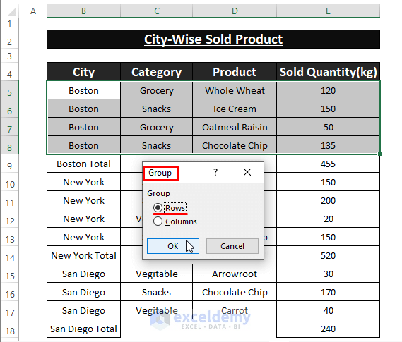
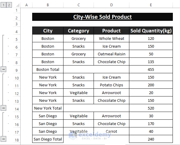
Excel makes a group from the selection.
- Repeat Steps 1 and 2 for other selections to get individual groupings for each selection.
Nested Grouping:
Steps:
- As above, perform Custom Sort and Subtotal for the different categories of data.
- Execute Single Grouping for each group.
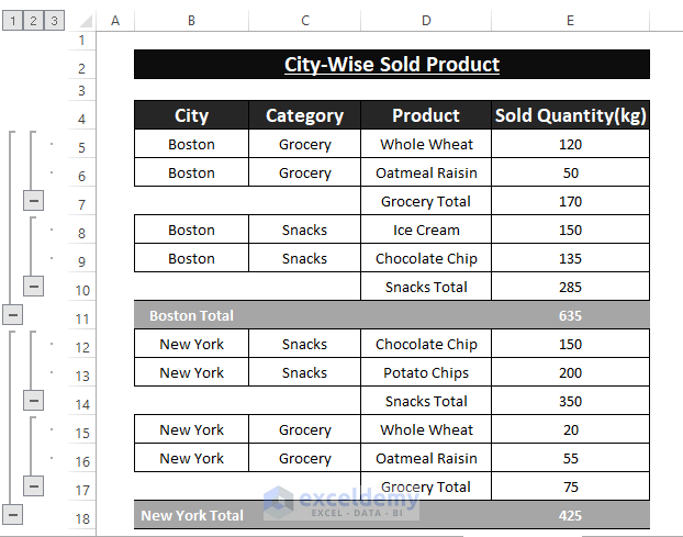
- For each different category section, execute the Data > Group process.
The result is something similar to the below picture.
Method 4 – Group Rows with Specific Entries Using Pivot Table
Pivot Table categorizes data in existing sections offering an overall synopsis of the data.
Steps:
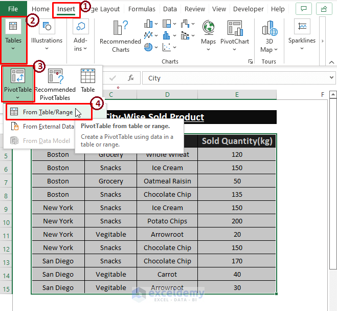
- Highlight the entire dataset.
- Go to the Insert tab.
- Click on Pivot Table (from Tables section).
- Click on From Table/Range.
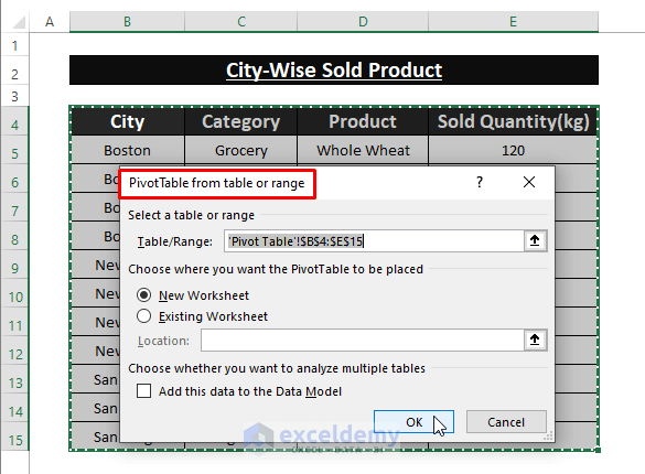
The PivotTable from table or range window opens.
- Choose New Worksheet as Choose where you want the PivotTable to be placed.
- Click on OK.
Excel loads PivotTable Fields in a new worksheet. In the new worksheet:
- Tick the necessary PivotTable Fields (City, Category, and Sold Quantity(kg)) to display in Rows.
- Display the Sum of Sold Quantity in the Values area.
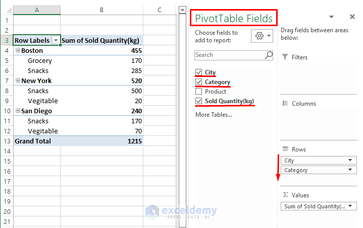
The Pivot Table groups the similar rows differentiating their Category too.
Read More: How to Group Rows in Excel by Name
Method 5 – Grouping Same Values Using Power Query in Excel
Similar to the Pivot Table, Power Query groups rows considering each entry along with the cells in a row. The Power Query Editor offers a Group By feature in its Home section.
Steps:
To open the Power Query Editor:
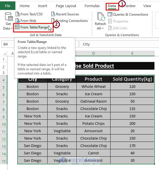
- Select the rows to group.
- Go to Insert.
- Click on From Table/Range (in the Get & Transform Data section).
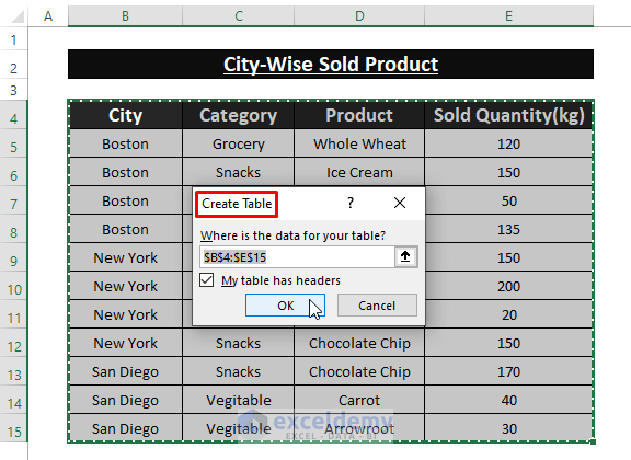
If your data is not in a Table, Excel brings up the Create Table dialog box.
- Tick My Table has headers.
- Click on OK.
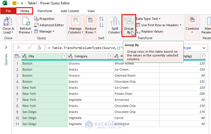
Excel creates a Table and opens Power Query Editor.
- Choose the Home section.
- Click on Group By.
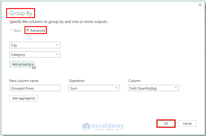
Excel opens the Group By dialog box.
- Add necessary grouping (Category) using the Add Grouping option.
- Assign a name (Grouped Rows) for the new column.
- Choose what Operation has to be performed (Sum).
- Assign a column (Sold Quantity(kg)) to execute the Sum Operation.
- Click on OK.
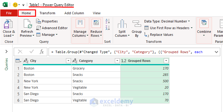
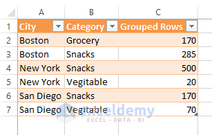
A new column with sorted rows depicting the Sum of each grouped row is created.
To load the data into a worksheet:
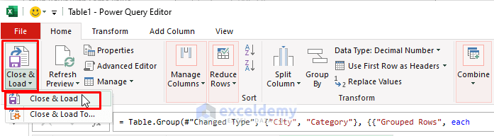
- Go to Close & Load.
- Click on Close & Load.
Excel loads the data as in the following image.
Method 6 – Group Rows with Certain Values Using INDEX-MATCH Formula
Condensing is an alternative way to group the rows. An INDEX-MATCH formula can condense rows with same value in just one row.
Steps:
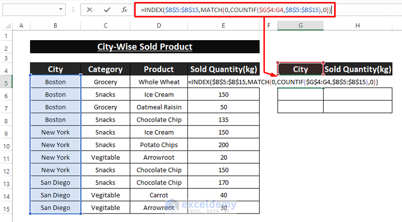
- Enter the following formula in any blank cell (G5) adjacent to the dataset:
=INDEX($B$5:$B$15,MATCH(0,COUNTIF($G$4:G4,$B$5:$B$15),0))The formula fetches a single entry of each similar entry from the $B$5:$B$15 array. $B$5:$B$15 = array, and MATCH(0,COUNTIF($G$4:G4,$B$5:$B$15),0) delivers the row_num for the INDEX function. The COUNTIF portion passes the lookup_array for the MATCH function.
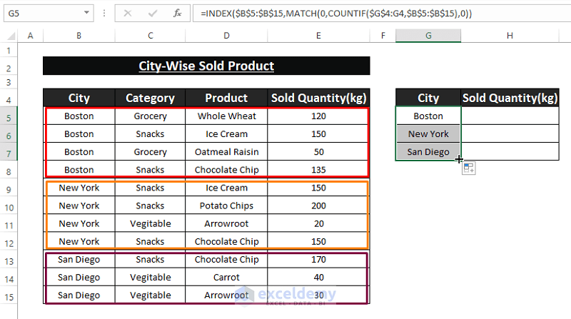
- Press ENTER and drag the Fill Handle to display each different entry within the given array.
The formula condenses the same entries into rows.
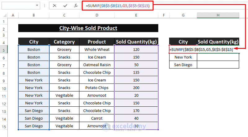
- Similarly, to aggregate the Sold Quantity for the same City, use the formula below in an adjacent cell (H5):
The SUMIF formula takes $B$5:$B$15 as range, G5 as Criteria, and $E$5:$E$15 as sum_range.
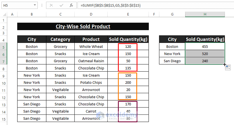
- Press ENTER to apply the formula.
- Drag the Fill Handle down to display each City’s total Sold Quantity.
Download Excel Workbook
Related Articles
- Group Rows with Plus Sign on Top in Excel
- How to Group Rows in Excel with Expand or Collapse
- How to Group Rows in Excel
- How to Group Columns Next to Each Other in Excel
<< Go Back to Group Cells in Excel | Outline in Excel | Learn Excel
Get FREE Advanced Excel Exercises with Solutions!
