How to Group Rows in Excel using the Expand or Collapse features – 5 Methods

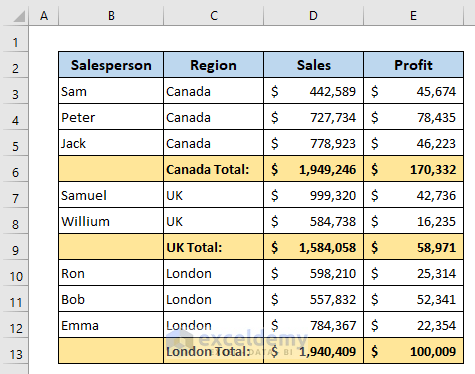
This is the sample dataset.

Method 1 – Using a Shortcut Key to Group Rows in Excel with the Expand or Collapse feature

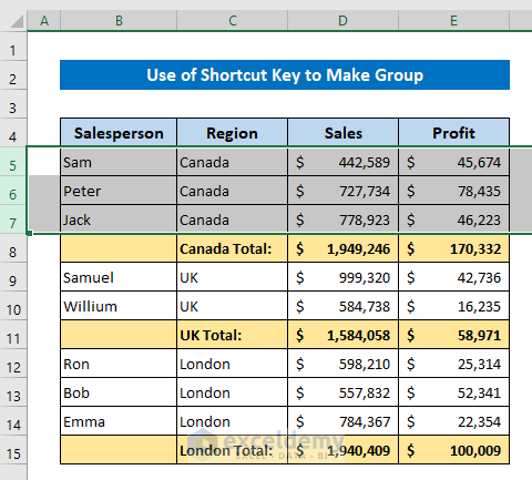
To group data for Canada:

• Select the rows that contain Canada.
• Press Shift+Alt+Right Arrow Key.

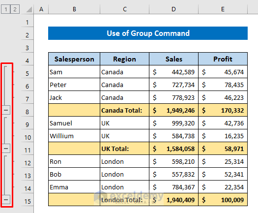
Rows are grouped with the expand or collapse option.

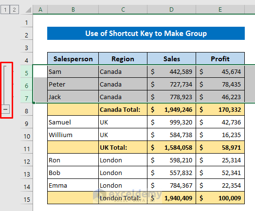
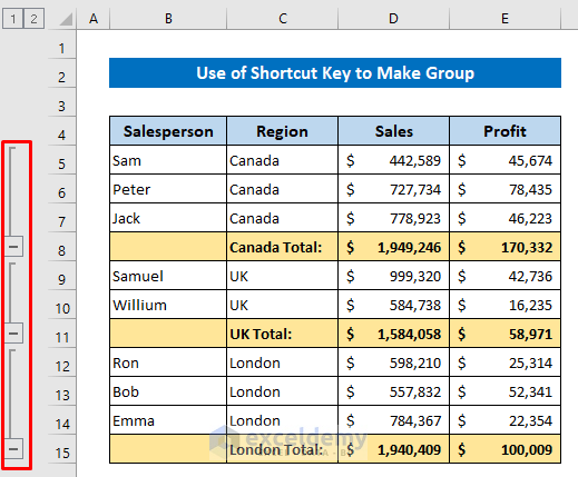
Apply the same procedure for the other regions.

Read More: How to Group Rows in Excel

Method 2 – Use the Group Command to Group Rows in Excel with the Expand or Collapse feature

• Select the rows containing Canada.
• Click: Data > Outline > Group

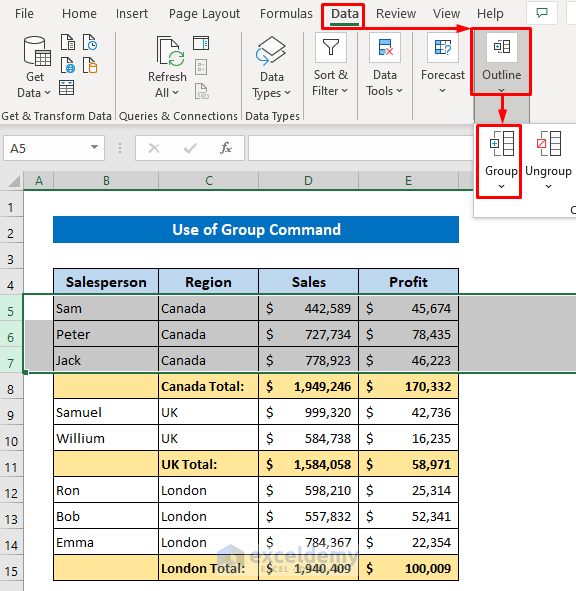
Follow the same steps for the other regions.

Read More: How to Group Rows by Cell Value in Excel

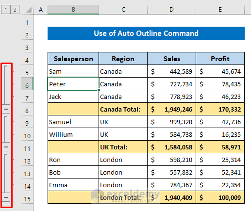
Method 3 – Use the Auto Outline Command to Group Rows in Excel with the Expand or Collapse feature

• Select any data in the dataset.
• Click: Data > Outline > Group > Auto Outline

Groups were created for different regions:

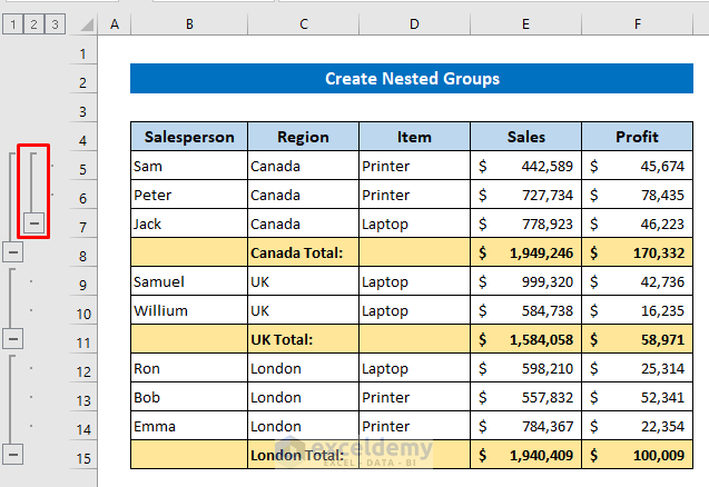
Method 4 – Create Nested Groups in Excel with the Expand or Collapse feature

A new column was added to show the selling items.

Group the printer items within Canada.

• Select the rows that contain Printer within the Canada group.
• Press Shift+Alt+Right Arrow Key or click Data > Outline > Group.

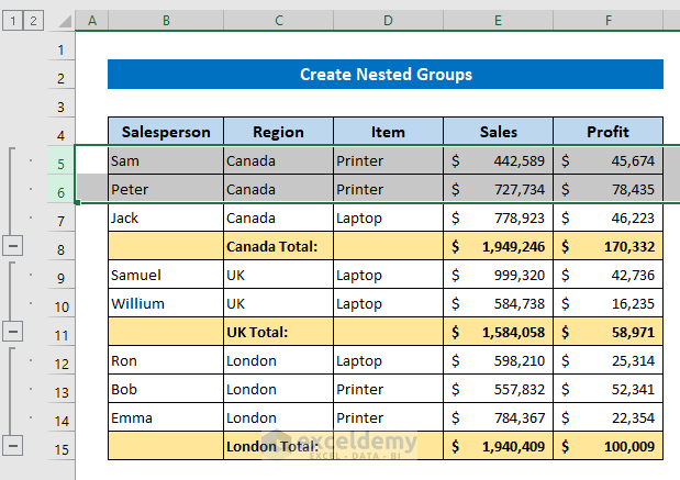
The nested group or subgroup is created.

Read More: How to Group Rows in Excel by Name

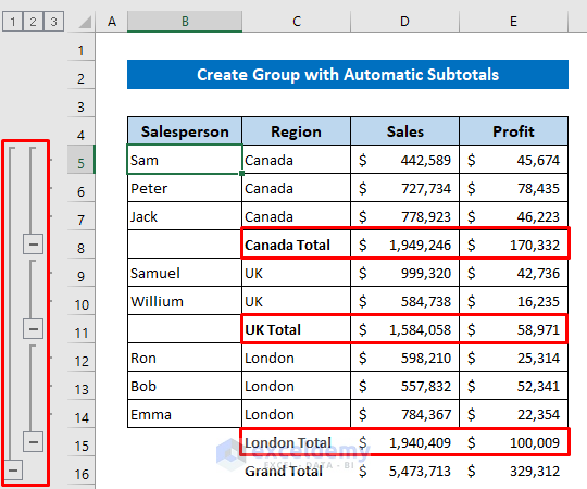
Method 5 – Create a Group with Automatic Subtotals in Excel

• Click any data in the dataset.
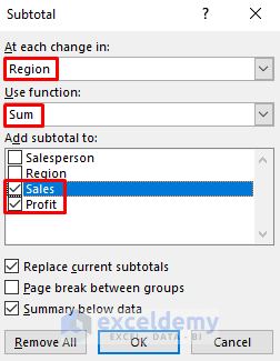
• Click: Data > Outline > Subtotal.

• Select Region in At each change in.
• Choose Sum in Use function.
• Check Sales and Profit in Add subtotal to.
• Click OK.

Groups and subtotals were created based on regions.

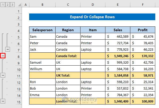
How to Expand or Collapse Rows in Excel

• To collapse groups, click the Minus sign at the lower part of each group.

You can  also do it using a command:

• Select data in the group you want to collapse.
• Click: Data > Outline > Hide Detail.

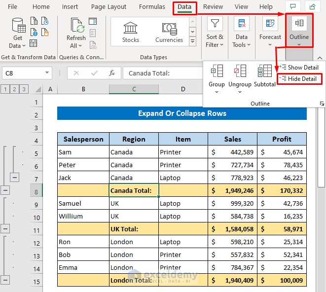
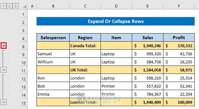
The group including the Canada region is collapsed and is showing a plus sign.

• To expand the group, click the plus sign.

• Or click: Data > Outline > Show Detail.

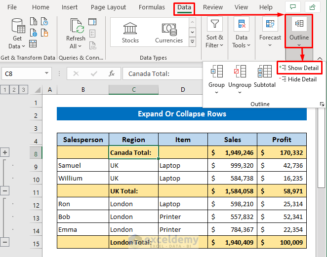
The group is expanded.

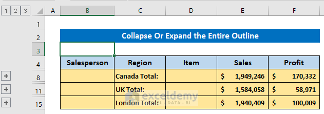
Collapse or Expand the Entire Outline 

If your dataset is very large, you can collapse or expand the entire outline at a time.

There are numbers above the expand/collapse option showing the group level.

The first level is the regions group. The second level is the items group within a region.

• Click 1 and all regions groups are collapsed.

This is the output.

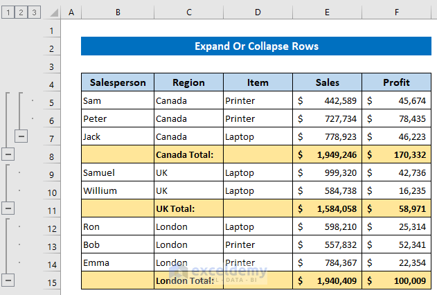
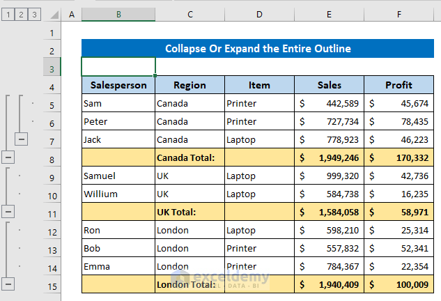
• To expand the entire outline, click 3.

All groups are expanded.

How to Remove an Outline and Ungroup Rows

• Select any cell in the dataset and click: Data > Outline > Ungroup > Clear Outline.

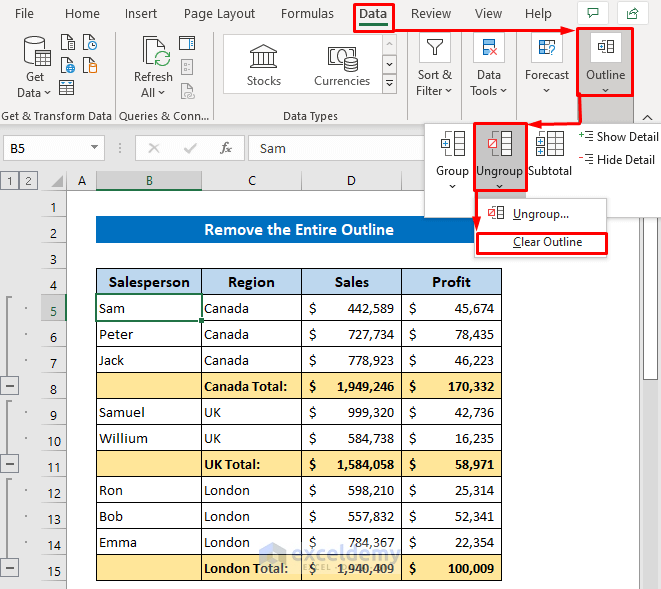
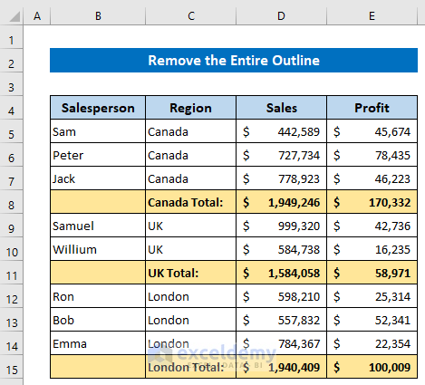
Excel removed the entire outline.

• To ungroup it, select the rows in the group and click: Data > Outline > Ungroup.

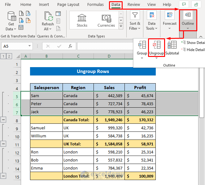
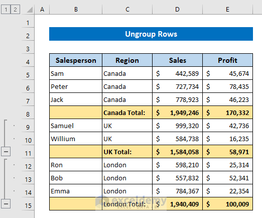
The rows are ungrouped.

Apply the same procedure for each group.

Read More: How to Group and Ungroup Columns or Rows in Excel

Things to Remember

• Press the right shortcut key: Shift + ALT + Right Arrow Key.
• The subtotal command is applied to sorted data.
• The Auto Outline command will group all the rows above the subtotal row.

Download Practice Workbook

Download the free Excel template.

Related Articles

• How to Group Rows with Same Value in Excel
• How to Group Columns Next to Each Other in Excel
• Group Rows with Plus Sign on Top in Excel

<< Go Back to Group Cells in Excel | Outline in Excel | Learn Excel