Method 1 – Group Time by Hour Intervals
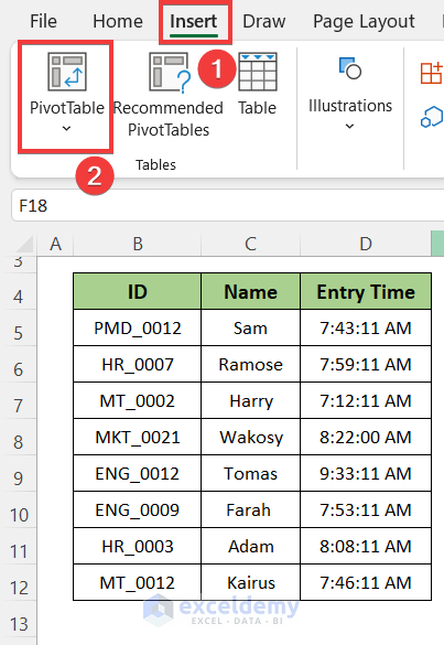
- Go to the Insert tab in the top ribbon.
- Click on the Pivot Table option.
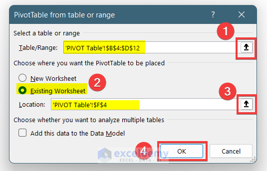
- Select the data from the worksheet by clicking on the arrow box in the Table/Range option.
- Select the Existing Worksheet option and select a cell to define where to start the pivot table.
- Press OK.
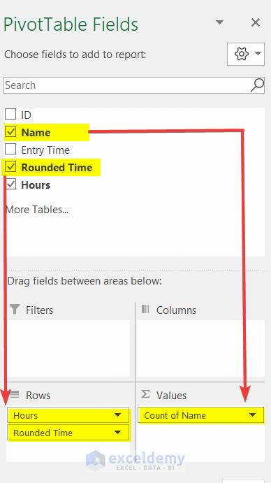
- See a Pivot Table will create in the worksheet and a “PivotTable Fields” window will appear on the right side of the worksheet.
- Drag the Entry time to the Rows section and Name to the Values section.
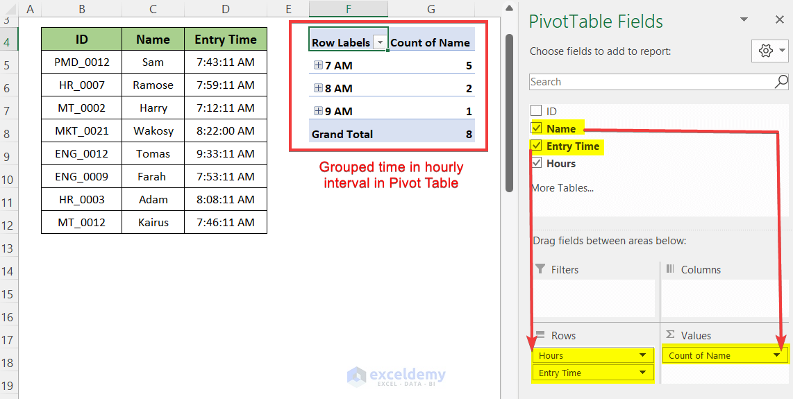
- You will see the pivot table is showing the numbers of people per hour interval.

Notes:
- The pivot table directly to the time column will work for 1 hour. If you want to take 30 minutes or any other you can’t make it.
- It makes intervals without rounding any time. It will take any time data in a range of 7:00:00 AM to 7:59:59 AM in the 7 AM range.
- Use this method to group time by hour intervals.
Method 2 – Group Time by Minute Intervals
2.1 Using FLOOR Function
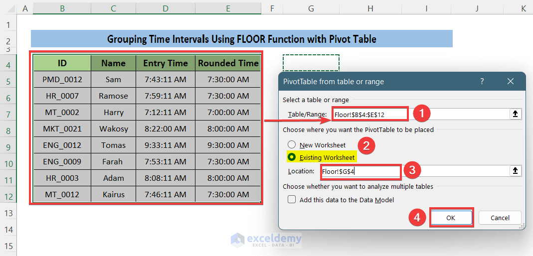
- Go to cell E5 and paste this formula to round the time to the nearest 30 minutes interval.
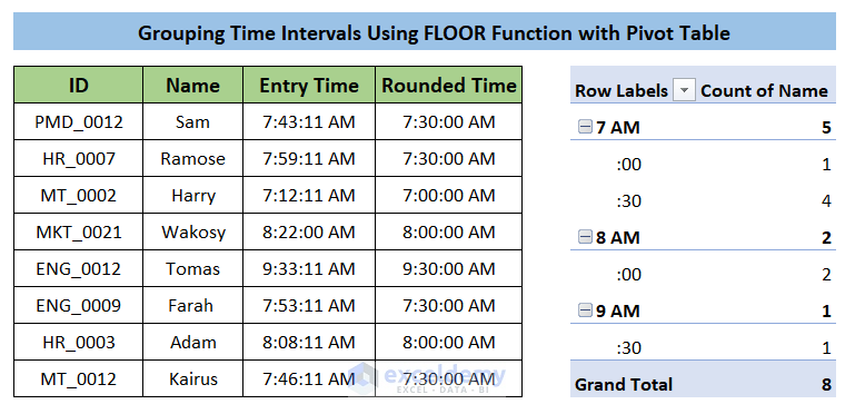
=FLOOR(D5,"0:30")- Drag the Fill Handle icon to paste the formula into the other cells or use Shortcuts Ctrl+C and Ctrl+P to copy and paste.
- The FLOOR function rounds the time to the nearest lower interval of the time.
- It rounds the time 7:43 AM to the nearest lower interval 7:30 AM
- The format to define interval here is “HH:MM: SS” so here “0:30” defines 0 hours 30 minutes interval.

- The rounded time groups the time into 30 minutes intervals. The rounded time describes a range of 30 minutes which starts from it. So, group 7:30 AM means a group range 7:30 AM to 8:00 AM
- Make a pivot table using the data in the existing worksheet by similar steps mentioned before.
- Drag the Rounded Time option into the Rows box and the Name option into the Values box.
- The pivot table will create and show the grouped data into 30 minutes intervals.
2.2 Using CEILING Function
You can also use the CEILING function to round the time to an interval.
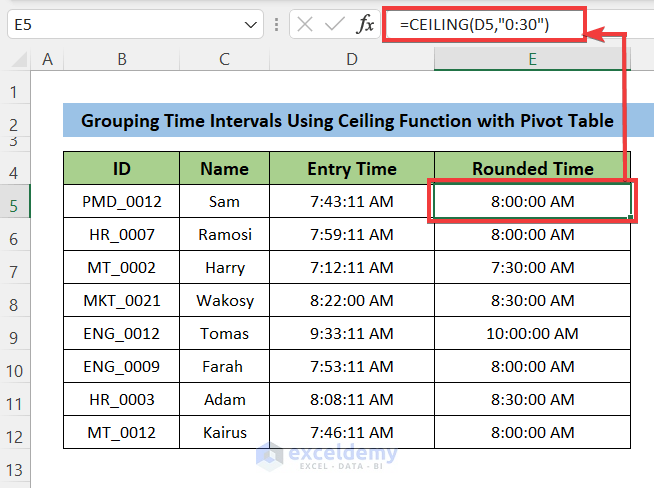
- Go to cell E5 and paste this formula to round the time to the nearest 30 minutes interval.
=CEILING(D5,"0:30")- Drag the Fill Handle icon to paste the formula into the other cells or use Shortcuts Ctrl+C and Ctrl+P to copy and paste.
- The CEILING function rounds the time to the nearest higher interval of the time.
- It rounds the time 7:43 AM to the nearest higher interval of 8.00 AM
- Make a pivot table for the data range. Then drag the rounded time into Rows and names into the Values box.
- You will see the pivot table will create and show grouped time data in 30 minutes intervals.
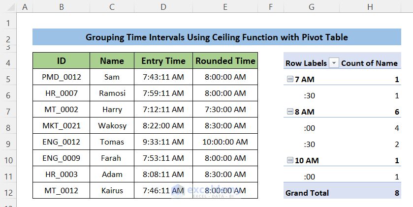
- The group 8:00 AM defines the range 7.30 AM to 8:00 AM.
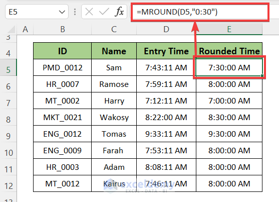
2.3 Using MROUND Function
The MROUND function rounds the time to the nearest interval. It doesn’t round to lower or higher intervals rather it rounds the time to that one which is the closest interval.
- Paste this formula into cell E5.
=MROUND(D5,"0:30")- Pull the Fill Handle icon to paste the formula into the other cells.
- The MROUND function rounds the time to the nearest interval of the time.
- It rounds the time 7:43 AM to the nearest higher interval of 8.00 AM and round time 7:12 AM to 7:10 AM
- Do the same things as mentioned in the Ceiling Function to create the pivot table.
- The time is grouped into 30 minutes intervals and shows the count of names in each group of intervals.

Notes:
MROUND function works differently than the FLOOR and CEILING function in grouping times for intervals as it rounds to the nearest intervals. For example, it rounds 7:59 AM to 8.00 AM also it rounds 8:08 AM to 8:00 AM. So, you can say for the 8:00 AM group the range is 7:45 AM to 8:15 AM.
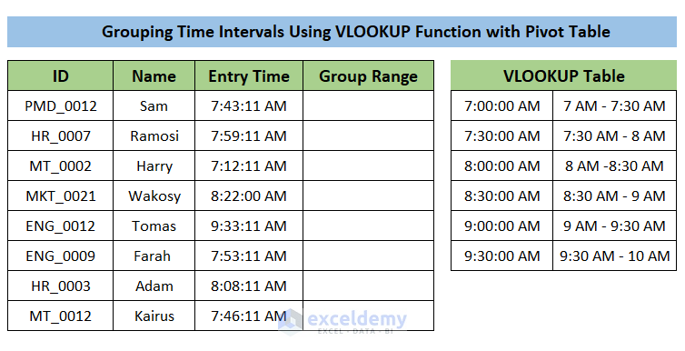
Method 3 – Group Time into Any Interval
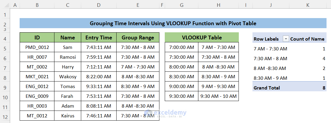
To remove confusion, you can use the VLOOKUP function to group time intervals where the intervals are described in a table.
- You have to make a table where the intervals are well-defined with the starting time of the interval.
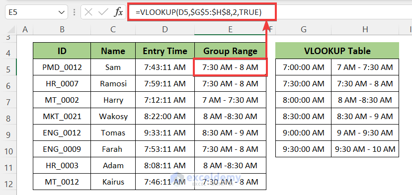
- Paste this formula into cell E5.
=VLOOKUP(D5,$G$5:$H$8,2,TRUE)- D5 – the lookup value for which the function will search the table.
- $G$5:$H$8 – The range where the lookup value locates. Use Absolute Reference so you can copy the formula to the other cells.
- TRUE – it will search for an approximate match of the look value. It will take the lower nearest interval from the table.
- Follow the steps to create the pivot table.
- The PivotTable Fields window, drag the “Group Range” into the Rows box and the names of the row to the values box.
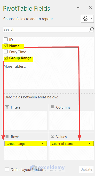
- The pivot table will create. And it is showing the total number of people for each group of the time interval.
Things to Remember
- Using a simple pivot table will give group data on hourly time intervals in Excel.
- You can use the FLOOR function to round the time to lower the nearest time interval. Using pivot table you can make the grouped data with time intervals where the group format is like 8:00 AM stands for the time interval 8:00 AM to 8:30 AM.
- And, the CEILING function rounds the time to the higher nearest time interval. So, here the 8:00 AM group will define the time interval from 7:30 AM to 8:00 AM.
- The MROUND function rounds the time to the nearest time interval. So, it makes groups like 8:00 AM mean the group 7:45 AM to 8:15 AM.
- The VLOOKUP function works with a ready group of time intervals.
Download Practice Workbook
You can download the practice workbook from here:
Related Articles
- How to Remove Grouping in Excel
- How to Use Grouping and Consolidation Tools in Excel
- How to Group Cells with Same Value in Excel
- How to Group Duplicates in Excel
- How to Group Similar Items in Excel
<< Go Back to Group Cells in Excel | Outline in Excel | Learn Excel
Get FREE Advanced Excel Exercises with Solutions!

